Dr. Neal, WKU
MATH 307
n
Linear Transformations
from Rn to Rm
m
n
m
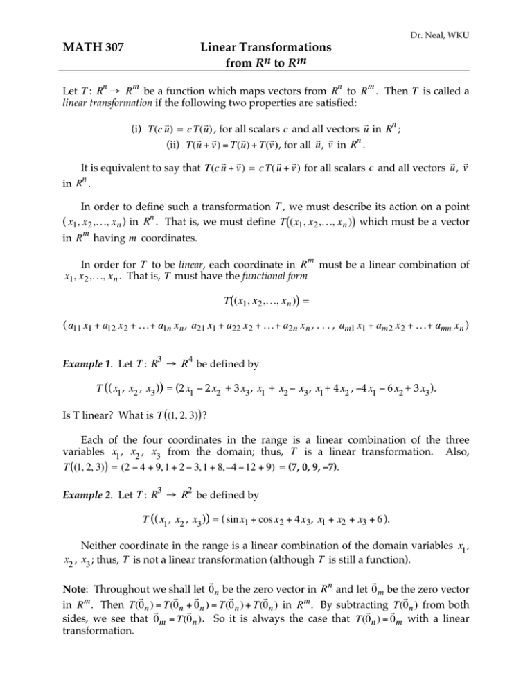
Let T : R → R be a function which maps vectors from R to R . Then T is called a
linear transformation if the following two properties are satisfied:



n
(i) T(c u) = c T( u) , for all scalars c and all vectors u in R ;
 
 


n
(ii) T( u + v ) = T( u) + T(v ) , for all u , v in R .
 
 
 
It is equivalent to say that T(c u + v ) = c T( u + v ) for €
all scalars c and all vectors u , v
€
€
n
in R .
€ €
€
In order to define such a transformation T , we must describe its action
on a point
€ €
€
n €
( x1, x 2 ,. . ., x n ) in R . That is, we must define T ((x1, x 2 ,. . ., x n )) which must be a vector
in R
m
having m coordinates.
m
In order for T to be linear, each coordinate
in R
€
x1, x 2 ,. . ., x n . That is, T must have the functional form
€
must be a linear combination of
T ((x1, x 2 ,. . ., x n )) =
€
( a11 x1 + a12 x 2 + . . . + a1n x n , a21 x1 + a22 x 2 + . . . + a2n x n , . . . , am1 x1 + am2 x 2 + . . . + amn x n )
€
3
4
Example 1. Let T : R → R be defined by
€
€
€
T (( x1 , x2 , x3 )) = (2 x1 – 2 x2 + 3 x3 , x1 + x2 – x3 , x1 + 4 x2 , –4 x1 – 6 x2 + 3 x3 ).
Is T linear? What is T ((1, 2, 3)) ?
Each of the four coordinates in the range is a linear combination of the three
variables x1 , x2 , x3 from the domain; thus, T is a linear transformation. Also,
T ((1, 2, 3)) = (2 − 4 + 9, 1 + 2 − 3, 1 + 8, –4 − 12 + 9) = (7, 0, 9, –7).
3
2
Example 2. Let T : R → R be defined by
T (( x1 , x2 , x3 )) = ( sin x1 + cos x 2 + 4 x 3, x1 + x2 + x3 + 6 ).
Neither coordinate in the range is a linear combination of the domain variables x1 ,
x2 , x3 ; thus, T is not a linear
€ transformation (although T is still a function).


Note: Throughout we shall let 0 n be the zero vector in R n and let 0 m be the zero vector






in R m . Then T(0 n ) = T(0 n + 0 n ) = T(0 n ) + T(0 n ) in R m . By subtracting T(0 n ) from both




sides, we see that 0 m = T(0 n ) . So it is always the case that T(0 n ) = 0 m with a linear
transformation.
€
€
€
€
€
€
€
€
€
Dr. Neal, WKU
The Matrix Representation
n
m
Every linear transformation T : R → R can be represented by a unique m × n matrix
A . The m rows are the coefficients from the linear combinations of the function form
m
n
m
coordinates in R . That is, suppose T : R → R is defined by
T ((x1, x 2 ,. . ., x n )) =
( a11 x1 + a12 x 2 + . . . + a1n x n , a21 x1 + a22 x 2 + . . . + a2n x n , . . . , am1 x1 + am2 x 2 + . . . + amn x n ),
€
 a11

 a21

then A =  .
 .

a
 m1
a12
a22
€
.
.
am2
.
.
.
.
.
.€ . a1n 

. . a2n 

. .
. .
. .
. 
. . am n 

If we let x = ( x1, x 2 ,. . ., x n ) ∈ R n , then we
 x1 
€
 
 x2 
 
€
€
 . €
can write X =   as an n × 1 matrix.
 .
 .
 
 xn 
The function value T ((x1, x 2 ,. . ., x n )) then can be computed by the matrix product
m
A X which gives an m × 1 matrix that is the function value point in R . We therefore

interchangeably write T( x ) = A X .
€
3
4
Example 3. Let T : R → R be defined by
€
T (( x1 , x2 , x3 )) = (2 x1 – 2 x2 + 3 x3 , x1 + x2 – x3 , x1 + 4 x2 , –4 x1 – 6 x2 + 3 x3 ).
 2 −2 3 


 1 1 −1
The matrix representation is the 4 × 3 matrix A = 
 . How do we evaluate
4 0
1


 −4 −6 3 
 2 −2 3 
 7
 1

  1  
 
 1 1 −1    0 
T ((1, 2, 3)) ? Let X =  2 , then T ((1, 2, 3)) = A × X = 
 ×  2 =   =
4 0    9
 
1
 3

  3  
 −4 −6 3 
 −7
4
(7, 0, 9, –7) as coordinates in R .
3
What is the action of T on the standard basis in R ?
Dr. Neal, WKU
 2 −2 3 
2

  1  
 1 1 −1    1 
We see that 
 ×  0 =   , and
4 0    1 
1
 −4 −6 3   0  −4


 
 2 −2 3 
 3

  0  
 1 1 −1    −1

 ×  0 =   .
4 0    0
1
 −4 −6 3   1  3 


 
 2 −2 3 
 −2

  0  
 1 1 −1    1 

 ×  1 =   , and
4 0    4 
1
 −4 −6 3   0  −6


 
Thus, the columns of A are simply the action of
T on the standard basis elements (1, 0, 0), (0, 1, 0),
and (0, 0 1). Therefore, each of the columns of A are
actually elements in the range of T .
A Matrix Defines a Linear Transformation
Reversing the process, we see that any m × n matrix A defines a linear transformation
n
m
T A : R → R by
 x1 
 
 x2 
 

 .
T A (x) = A X , where x = ( x1, x 2 ,. . ., x n ) and X =   .
 .
 .
 
 xn 
€ €
 3 −2 8 
 , then T A : R3 → R2 is defined by
For example, given the 2 × 3 matrix A = 
 4 6 −3
 x1 
 3 −2 8 
 × x 
T (( x1 , x2 , x3 )) = 
 4 6 −3  2 
 x3 
 3x1 − 2x 2 + 8x3 
=
= ( 3x1 − 2x2 + 8x3 , 4x1 + 6x2 − 3x3 ).
 4x1 + 6x2 − 3x3 
Defining T by Action on the Standard Basis
n
m
T : R → R can also be defined by its action on the standard
A linear transformation


basis. Let e1 = (1, 0, . . ., 0) , e2 = (0, 1, . . ., 0) , . . . , en = (0, 0, . . ., 1) . If we know what T
does to each basis element, then we can evaluate T at any point.
Because T is linear, we have
€ T ((x , x ,. . ., x €)) = T ( x e + x e + . . .€+ x e ) = x T(e ) + x T(e ) + . . . + x T(e ) .
1 2
n
1 1
2 2
n n
1
1
2
2
n
n
€
Also, once we know the action on the standard basis, then we also know the
columns of the matrix representation A ; thus, we can easily evaluate T at any point.
€
€
Dr. Neal, WKU
4
3
Example 4. Evaluate T ((−2, 3, 8, − 10)) for T : R → R defined by
T ((1, 0, 0, 0)) = (−1, 2, − 3)
T ((0, 0, 1, 0)) = (1, 2, 4)
T ((0, 1, 0, 0)) = (2, − 1, 4)
T ((0, 0, 0, 1)) = (−2, 0, 6) .
Solution. Because T is linear, we have
T ( (−2, 3, 8, − 10) ) = −2 T ( (1, 0, 0, 0) ) + 3 T ((0, 1, 0, 0)) + 8 T ( (0, 0, 1, 0) ) − 10 T ( (0, 0, 0, 1) )
= −2 (−1, 2, − 3) + 3 (2, − 1, 4) + 8 (1, 2, 4) − 10 (−2, 0, 6) = (36, 9, − 10) .
 −1 2 1 −2
Or we can write A =  2 −1 2 0  , where the columns of A are the action on

 −3 4 4 6 
 −2 
 −1 2 1 −2
 36 
 3 
the st. basis. Then T ((−2, 3, 8, − 10)) =  2 −1 2 0  × 
=  9  = (36, 9, − 10) .


 
8
  −10
 −3 4 4 6  
 −10
One-to-One Transformations
n
m
Let T : R → R be a linear transformation. Then T is one-to-one (or injective) if it is
always the case that different values
are assigned to different values in

in the domain

the range. That is, whenever u ≠ v then T( u) ≠ T(v ) . By the
 contrapositive, it is
logically equivalent to say that whenever T( u) = T(v ) , then u = v .


To prove that a function is one-to-one, we often assume that T( u) = T(v ) and then
€ €

€
€
T from Rn to R m , we can use
argue that u must equal v . With a linear transformation
€
€
€
€
the following results to check if T is one-to-one:
€
€
€
€
n
m
A.
Theorem 2.1. Let T : R → R be a lineartransformation with matrix representation
 

Then T is one-to-one if and only if T( z ) = 0 m has only the trivial solution of z = 0 n .
€


Proof. We know that T(0 n ) = 0 m for any linear transformation. Suppose first that T is
 
 
one-to-one. If T( z ) = 0 m also, then z = 0 n because T is one-to-one.€
€
 €
 
Now suppose that z = 0 n is the onlysolution of T( z ) = 0 m . To prove that T is one

 


to-one, assume
that T( x ) = T( y ) . Then 0 m = T( x ) – T( y ) = T( x − y ) which means that
€
  
 
T is one-to-one.
QED
x − y =€0 n . Hence, x = y and
€ €
€ €
€
€
€
€
€
€
€
€ matrix equations, Theorem 2.1 is equivalent to saying that T is one-to-one
Note: Using
if and only if the homogeneous system A X = 0 has only the trivial solution of X = 0.
Dr. Neal, WKU
n
m
Theorem 2.2. Let T : R → R be a linear transformation with matrix representation A .
If m < n , then T cannot be one-to-one.
n
m
Proof. Note: Because R is a “larger” set than R when m < n , it should not be possible
n
m
to map R to R in a one-to-one fashion.
To prove the result, observe that the matrix representation A will be an m × n
matrix with fewer rows than columns. Thus the last (non-zero) row of the reduced row
echelon form of the homogeneous system A 0 will have independent (or free)
variables. Hence A X = 0 will have infinite solutions (not just the trivial solution). By
Theorem 1, T cannot be one-to-one.
1 0 . . .

0 1 . . .

. . 1 . .
. . . 1 .

0 . . . 1

n
. .
. .
. .
. .
. cn
0

0

.
. 
0
m
Theorem 2.3. Let T : R → R be a linear transformation with matrix representation A .
Assume m > n . Then T is one-to-one if and only if the reduced row echelon form of A
reduces to the n × n identity with additional rows that are all 0.
Proof. To determine if T is one-to-one, we must see if the homogeneous system A X = 0
has only the trivial solution. We consider the reduced row echelon form of the m × n
matrix A . Because there are more rows than columns, we have two cases:
 1 . . . 0


. 1 . . .


. . 1 . .
. . . 1 .


 0 . . . 1


 0 . . . 0
the n × n identity with
additional rows that are all 0
 1 . . . c1 


. 1 . . . 


 . . 1 . cn 
0 . . . 0 


. . . . . 


0 . . . 0 
free variables remain in the
last non-zero row
In the first case, A X = 0 has only the trivial solution; thus, T is one-to-one. In the
second case, A X = 0 has infinite solutions; thus, T is not one-to-one.
n
n
Theorem 2.4. Let T : R → R be a linear transformation with matrix representation A .
Then T is one-to-one if and only if det (A) ≠ 0.
Proof. Because A is now n × n , we can say det (A) ≠ 0 if and only if the homogeneous
system A X = 0 has only the trivial solution if and only if T is one-to-one.
Dr. Neal, WKU
3
4
Example 5. Let T : R → R be defined by
T (( x1 , x2 , x3 )) = (2 x1 – 2 x2 + 3 x3 , x1 + x2 – x3 , x1 + 4 x2 , –4 x1 – 6 x2 + 3 x3 ).
Is T one-to-one?
Solution. We let A be the matrix representation and look at the reduced row echelon
form of homogeneous system A 0 :
 2 −2 3 0
1



1
1 −1 0
0

 → rref → 
4 0 0
1
0
 −4 −6 3 0
0



0
1
0
0
0
0
1
0
0

0

0
0
The only solution to A X = 0 is X = 0; thus, T is one-to-one. ( A reduces to the
identity with an additional row of 0's.)
4
5
Example 6. Let T : R → R be defined by
T ((1, 0, 0, 0)) = (−1, 2, − 3, 0, 1)
T ((0, 0, 1, 0)) = (1, 2, 4, 0, 2)
T ((0, 1, 0, 0)) = (2, − 1, 4, 1, 0)
T ((0, 0, 0, 1)) = (2, 6, 3, 2 , 5) .
Is T is one-to-one?
Solution. We look at the reduced row echelon form of homogeneous system A 0 :
 −1 2 1 2 0
1 0



 2 −1 2 6 0
0 1



 −3 4 4 3 0 → rref →  0 0
 0 1 0 2 0
0 0



 1 0 2 5 0
0 0



0
0
1
0
0
3
2
1
0
0
0

0

0
0
0
We see that A X = 0 has infinitely many solutions; thus, T is not one-to-one.
(Matrix A does not reduce to the identity with additional rows of 0.)
2
2
Example 7. Let T : R → R be the reflection about the x -axis. Is T one-to-one?
1 0 

Solution. We define T by T ((x, y)) = (x, − y) . The matrix representation is A = 
 0 −1
(which are the coefficients from the linear combinations of the function form
coordinates). Because det (A) = –1 ≠ 0, we see that T is one-to-one.
Dr. Neal, WKU
Onto Transformations
n
€
€
m
Let T : R → R be a linear transformation. Then T is onto (or surjective) if every vector



b ∈ R m has a pre-image in Rn . That is, for every
b
∈ R m there is a vector v ∈R n such




that T(v ) = b . (The vector v is a pre-image of b .) That is, the equation T( x ) = b always

has a solution for every b ∈ R m .
€
€
€
€
€
€
€
We can use the following results to determine if a linear transformation
is onto:
€
n
m
Theorem 2.5. Let T : R → R be a linear transformation with matrix representation A .
Then T is onto if and only if the matrix equation A X = B always has a solution for
every m × 1 matrix B .


Proof. Because the equation T( x ) = b is equivalent to the matrix equation A X = B , the
theorem is simply a matrix form re-statement of the definition of “onto.”
€m
€ n
Theorem 2.6. Let T : R → R be a linear transformation with matrix representation A .
If m > n , then T cannot be onto.
m
n
Proof. Note: Because R is a “larger” set than R when m > n , it should not be
m
possible for every element in R to have a pre-image by means of the function T .
To prove the result, observe that the matrix representation A will be an m × n
matrix with more rows than columns. Thus the reduced row echelon form of any
system A B will have the additional rows in A become all 0. These rows will lead to
inconsistencies for certain m × 1 matrices B . Thus A X = B will not always have a
solution and T cannot be onto.
1 .

0 1

. .
. .

0 0

. . c1 

. . c2 

1 . . 
. 1 . 
0 0 cm 
n
m
Theorem 2.7. Let T : R → R be a linear transformation with matrix representation A .
Assume m < n . Then T is onto if and only if the reduced row echelon form of A does
not contain a row of all 0's.
Proof. To determine if T is onto, we must see if every possible system A X = B has a
solution. We consider the reduced row echelon form of the m × n matrix A . Because
there are fewer rows than columns, we have two cases:
Dr. Neal, WKU
 1 0 . . . . .


 0 1 . . . . .


 . . 1 . . . .
 . . . 1 . . .




 0 . . . 1 . .
no rows become all 0
 1 0 . . . . .


 0 1 . . . . .


 . . 1 . . . .
 . . . 1 . . .




 0 0 . . . . 0
a row becomes all 0
If no rows become all 0, then there will never be an inconsistency. So A X = B will
always have a solution and T is onto.
If a row becomes all 0, then there will be inconsistencies for some B when trying to
solve A X = B . Thus at times A X = B will have no solution and T will not be onto.
n
n
Theorem 2.8. Let T : R → R be a linear transformation with matrix representation A .
Then T is onto if and only if det (A) ≠ 0.
Proof. Because A is now n × n , we can say det (A) ≠ 0 if and only if any system A X = B
always has a solution if and only if T is onto.
n
n
Theorem 2.9. Let T : R → R be a linear transformation. Then T is either both one-toone and onto (i.e., a bijection), or T is neither one-to-one nor onto.
Proof. Let A be the matrix representation of T . By Theorems 4 and 8, T is one-to-one if
and only if det (A) ≠ 0 if and only if T is onto. Thus T is one-to-one if and only if T is
onto. That is, T is either both one-to-one and onto, or T is neither one-to-one nor onto.
4
3
Example 8. Let T A : R → R be defined by the matrix representation
 1 0 −2

A =  1 −2 1

 −2 1
0
4

−3

2
where T A (x) = A X . Is T A one-to-one and/or onto? Is the point (4, –2, 6) in the range of
T A ? If so, find a pre-image.
3
4
Solution. Because R is a “smaller” set than R , T A cannot be one-to-one (Theorem 2).
To determine if T A is onto, we consider the reduced row echelon form of A :
 1 0 0 −1.2 


 0 1 0 −0.4


 0 0 1 −2.6
Dr. Neal, WKU
Because no rows became all 0, there will never be an inconsistency. So every system
A X = B will have a solution; therefore, T A is onto.


3
b
∈
R
v
∈ R 4 such that
Now
we
can
say
that
for
any
vector
,
there
is
a
pre-image


T(v ) = b . (In fact we can see from rref( A ) that there will be infinite pre-images, which
also verifies that T A is not one-to-one.)

In particular, we can solve the
€ equation TA ( x ) = (4, –2, 6): €
€
€
1
0 −2
 1 −2 1

 −2 1
0
4 4
€→
−3 −2 → rref

2 6
1 0
0 1

0 0
x1 = −4.8 + 1.2 t
0 −1.2 −4.8
x2 = −3.6 + 0.4 t
0 −0.4 −3.6 →

x3 = −4.4 + 2.6 t
1 −2.6 −4.4
x4 = t
If t = 0, then (–4.8, –3.6, –4.4, 0) is one particular pre-image of (4, –2, 6). That is,
T ((−4.8, − 3.6, − 4.4, 0)) = (4, –2, 6).
3
4
3
Example 9. Let T : R → R be the “embedding” map which places a point from R into
R 4 by adding a 0 in the 4th coordinate. Is T one-to-one and/or onto?
Solution. Here we can define T by T ((x, y, z)) = (x, y, z, 0) . The matrix representation is
 1 0 0


 0 1 0
the 4 × 3 matrix A = 
 . We see that A is already in rref form and has a row of
 0 0 1
 0 0 0


4
all 0's. By Theorem 7, T is not onto. (In particular, every element in R with a non-zero
4th coordinate will cause an inconsistency; thus, these elements will not be in the
range.) However, the homogeneous system A X = 0 has only the trivial solution of X =
0; thus, T is one-to-one.
n
n
Inverses of Transformations from R to R
n
n
When a linear transformation T : R → R is both one-to-one and onto, then we can
−1
n
n
find the inverse transformation T : R → R such that if T ((x1, x 2 ,. . ., x n )) =
(y1, y2 ,. .., yn ) , then T −1((y1, y2 ,. . ., yn )) = ( x1, x 2 ,. . ., x n ).
€
If A is the matrix representation of the one-to-one and onto T , then we know that
€
−1
det (A) ≠ 0. Therefore A exists. Because T ((x1, x 2 ,. . ., x n )) = (y1, y2 ,. .., yn ) is equivalent
to A X = Y , we can apply the matrix inverse and say that X = A −1 Y . Thus, A
−1
be the matrix representation of T because ( x1, x 2 ,. . ., x n ) = T −1((y1, y2 ,. . ., yn )) .
€
€
−1
must
Dr. Neal, WKU
3
3
Example 10. Let T : R → R be defined by
T ((1, 0, 0)) = (1, 0, –1)
T ((0, 1, 0)) = (2, 1, 2)
Verify that T is a bijection. Find the function form of T
−1
T ((0, 0, 1)) = (1, 1, 4)
.
 1 2 1
Solution. The matrix representation of T is A =  0 1 1 and det (A) = 1 ≠ 0; thus T

 −1 2 4
is both one-to-one and onto (i.e., a bijection). The matrix representation of T
 2 −6 1 
 −1 5 −1 . Thus,


 1 −4 1 
−1
is A
−1
=
T −1((x, y, z)) = (2x − 6y + z, − x + 5y − z, x − 4y + z) .
Note: T −1((1, 0, − 1)) = (1, 0, 0) , T −1((2, 1, 2)) = (0, 1, 0), and T −1((1, 1, 4)) = (0, 0, 1).
2
2
−1
Example 11. Let T : R → R be the reflection about the x -axis. Find T .
1 0 
1 0 
 . Then A −1 = 
 also. So
Solution. Here T ((x, y)) = (x, − y) and A = 
 0 −1
 0 −1
T −1((x, y)) = (x, − y) = T ((x, y)) . In other words, T is its own inverse. If you reflect
about the x -axis, then you “undo” the process by reflecting back about the x -axis.
Null Space and Nullity
n
€
€
m
Let T : R → R be a linear transformation, with m × n matrix representation A . The
 

null space (or kernel of T ) is the set of all vectors x ∈ R n such that T( x ) = 0 m . We know


that T(0 n ) = 0 m . If T is one-to-one,
then no other vector gets mapped to the origin; so

the null space is simply { 0 n }.
But if T is not one-to-one, then AX =
many solutions as will
€ 0 will have infinitely
€
 
T( x ) = 0 m . The set of all solutions to AX = 0 is called the null space. The nullity is the
dimension of this null space and is given by the number of independent parameters ( r ,
s , t , etc.) used €
in writing the form of all solutions to AX = 0 . And if T is one-to-one,
then the nullity is simply 0.
Dr. Neal, WKU
Range and Rank


 
The range of T is the set of all vectors y ∈ R m for which T( x ) = y for some x ∈ R n . All
of the columns in the matrix representation A are actually elements in the range of T .
The first column in A is the value T ((1, 0, 0, . . ., 0)) , the second column in A is the
value T ((0, 1, 0, . . ., 0)) , etc. But some of these columns may be linear combinations of
€ independent of €
€
the previous columns. The columns
in A that are
each other create the
T
T
dimensions in the range of . The actual range of will be the collection of all linear
combinations of these independent vectors, and the rank of T is the dimension of this
range.
5
5
Example 12. Let T : R → R be defined by its action on the standard basis as

T(e1 ) = (1, 1, 2, 0, 1)

T(e2 ) = (0, −1, −1, −1, 1)

T(e4 ) = (1, 1, 2, 0, 0)
€
(a)
(b)
(c)
(d)
(e)

T(e3 ) = (0, 1, 1, 1, −1)

T(e5 ) = (1, 0, 1, −1, 1)
€
Give the matrix representation
and functional €
form of T .
Is T one-to-one and/or onto?

€
Are b = (1, 2, 3, 4, 5) and c = (4, 2, €
6, –2, 5) in range of T ? If so, find pre-images.
Find the null space and nullity. Give a basis for the null space.
Find the range and rank.
€Solution. (a) The columns
€
of the matrix representation are the action on the standard
basis elements. Thus,
1

1

A = 2
0

1
0
0
−1 1
−1 1
−1 1
1 −1
1 1

1 0
2 1 
0 −1

0 1
T (( x1 , x2 , x3 , x4 , x5 )) =
( x1 + x4 + x5 , x1 – x2 + x3 + x4 , 2 x1 – x2 + x3 + 2 x4 + x5 , – x2 + x3 – x5 , x1 + x2 – x3 + x5 )
(b) det (A) = 0 ; thus, A is neither one-to-one nor onto.
(c)
€
1

1

A B = 2
0

1
0
−1
−1
0
1
1
1
1
2
1 1 4
1


0 2 2
0

1 3 6  rref →  0
0
−1 1 0 −1 4 −2 


1 −1 0 1 5 5 
0
0 0 0
1 −1 0
0 0 1
0
0
0
0
0
0
0 0 3

1 0 2
1 0 1 
0 1 0 

0 0 0

For b = (1, 2, 3, 4, 5), we see that AX = B has no solution,
 so (1, 2, 3, 4, 5) is not in the
range of T . However, there are infinite solutions for c = (4, 2, 6, –2, 5). One such
solution is (3, 2, 0, 1, 0). That is, c = (4, 2, 6, –2, 5) is in range of T and T ((3, 2, 0, 1, 0)) =
(4, 2, 6, –2, 5).
€
€
Dr. Neal, WKU
1

0

(d) rref (A 0) =  0
0

0
0
1
0
0
0
0
−1
0
0
0
0
0
1
0
0
0
1
1
0
0
0

0
0 
0 

0
The null space is all vectors of the form
(x1 , x2 , x3 , x4 , x5 ) = (0, s − t , s , − t , t )
where s and t are any real numbers.
It is 2-dimensional (using two variables),
so nullity = 2.
€
Letting (s, t) be (1, 0) then (0, 1), we obtain the€two vectors


v1 = (0, 1, 1, 0, 0) and v 2 = (0, –1, 0, –1, 1)
€Then any vector in the null space has the form s v1 + t v2 , which is a linear combination
 
 
of {v1, v 2 } . So {v1, v 2 } is then a basis for the null space.
€
€
(e) From rref (A) , we see that the original first, second, and fourth columns create the
€ of T will have three dimensions T .
3 × 3 identity in the rref. Thus, the range
€
Thus, rank T = 3 and the range of T is the collections of all linear combinations of the
three vectors T(e1 ) = (1, 1, 2, 0, 1) , T(e2 ) = (0, −1, −1, −1, 1) , and T(e4 ) = (1, 1, 2, 0, 0) , which
are the first, second, and fourth columns in the origianl matrix.
In other words, if we look at just the original first, second, and fourth columns as
vectors in R 5, then any vector in the range of T can be
 written as a linear combination
€
€
€
of justthese three vectors after rref is performed. For c = (4, 2, 6, –2, 5) as in Part (c), we



have c = 3 T(e1 ) + 2T(e2 ) + 1T(e4 ) .
€
€
€
Note:
Another way to label “all linear combinations of a collection of vectors” is to
€ the preceding example, the null space is
simply call
it the “span” of these vectors.
In



€ span
€ {v1, v€2 } and the
€ range is span{ T(e1 ) , T(e2 ) , T(e4 ) }.
Here is a description of the preceding transformtation:
€
€
€
5
5
T€
: R → R



Let e1 = (1, 0, 0, 0, 0) , e2 = (0,1, 0, 0, 0) , e4 = (0, 0, 0,1, 0) .
5
Domain: R
(5 dimensions)
€
  
span{ e1, e2 , e4 }
€
⊕
€ € €
Two-dimensional
 Null Space
span {v1, v 2 }
€
€
Range:
5
A Three Dimensional Subpace of R



span{ T(e1 ) , T(e2 ) , T(e4 ) }
→
T
→
∪
€
€ {0, €
0, 0, 0, 0}
5
T is not one-to-one: Two dimensions of R all get mapped to {0, 0, 0, 0, 0}.
€
T is not onto: The range is 3-d; only three dimensions of R5 have pre-images.
Dr. Neal, WKU
MATH 307
Linear Transformations: Rn to Rn
Exercises
3
3
1. Let T : R → R be defined in functional form by
T (( x1 , x2 , x3 )) = ( x1 – 2 x2 + 2 x3 , 2 x1 + x2 + x3 , x1 + x2 ).
(a)
(b)
(c)
(d)
Write the matrix representation A .
Prove that T is both one-to-one and onto.
Evaluate T ((–4, 6, 1)).
Find a pre-image of the point (–5, 3, 2);
i.e., solve the equation T (( x1 , x2 , x3 )) = (–5, 3, 2).
(e) Give both the matrix representation and the functional form of T
−1
.
4
4
2. Let T : R → R be defined by
T ((1, 0, 0, 0)) = (1, 2, 3, 1)
T ((0, 0, 1, 0)) = (–2, –4, 1, 4)
T ((0, 1, 0, 0)) = (3, 6, 9, 3)
T ((0, 0, 0, 1)) = (4, 8, 5, 8).
(a) Write the matrix representation A .
(b) Prove that T is neither one-to-one nor onto.
(c) Evaluate T ((–4, 6, 1, 2)).
(d) Determine if the points (5, 10, 8, 49) and (6, –4, 12, 20) are in the range of T , and if
so find pre-images of these points.
(e) Give the form of the null space and give the nullity of T . Also give a basis for the
null space.
(f) Describe the range of T and give the rank of T .
(g) Explain how the domain is divided into subspaces and how these subspaces are
4
mapped into R via T .
Dr. Neal, WKU
MATH 307
Linear Transformations: Rn to Rm
Exercises
6
4
1. Let T : R → R be defined by
T (( x1 , x2 , x3 , x4 , x5 , x6 )) =
(– x1 + 2 x2 + 4 x4 + 5 x5 – 3 x6 , 3 x1 – 7 x2 + 2 x3 + x5 + 4 x6 ,
2 x1 – 5 x2 + 2 x3 + 4 x4 + 6 x5 + x6 , 4 x1 – 9 x2 + 2 x3 – 4 x4 – 4 x5 + 7 x6 )
(a) Give the matrix representation of T .
(b) Determine and explain whether or not T is onto.
(c) Describe the range of T and give the rank of T .
(d) Determine and explain whether or not T is one-to-one.
(e) Give the form of the null space and give the nullity of T . Also give a basis for the
null space.
(f) Explain how the domain is divided into two subspaces and how these subspaces are
4
mapped into R via T .
5
3
2. Let T : R → R defined by matrix representation
1 4 5 0 9 


A =  3 −2 1 0 −1


2 3 5 1 8 
(a) Give the function form of T .
(b) Determine and explain whether or not T is onto.
(c) Describe the range of T and give the rank of T .
(d) Determine if (3, 2, 1) is in the range of T . If so, give a pre-image.
(e) Determine and explain whether or not T is one-to-one.
(f) Give the form of the null space and give the nullity of T . Also give a basis for the
null space.
3
4
3. Let T : R → R be defined by
T ((1, 0, 0)) = (3, 1, 0, 1)
T ((0, 1, 0)) = (1, 2, 1, 1)
T ((0, 0, 1)) = (–1, 0, 2, –1)
(a) Give the matrix representation of T .
(b) Evaluate T ((1, 2, 3)) .
(c) Determine and explain whether or not T is onto.
(d) Describe the range of T and give the rank of T .
(e) Determine if (1, 0, 0, 0) is in the range of T . If so, give a pre-image.
(f) Determine and explain whether or not T is one-to-one.
(g) Give the form of the null space and give the nullity of T . Also give a basis for the
null space.