4.1 Simple random variables
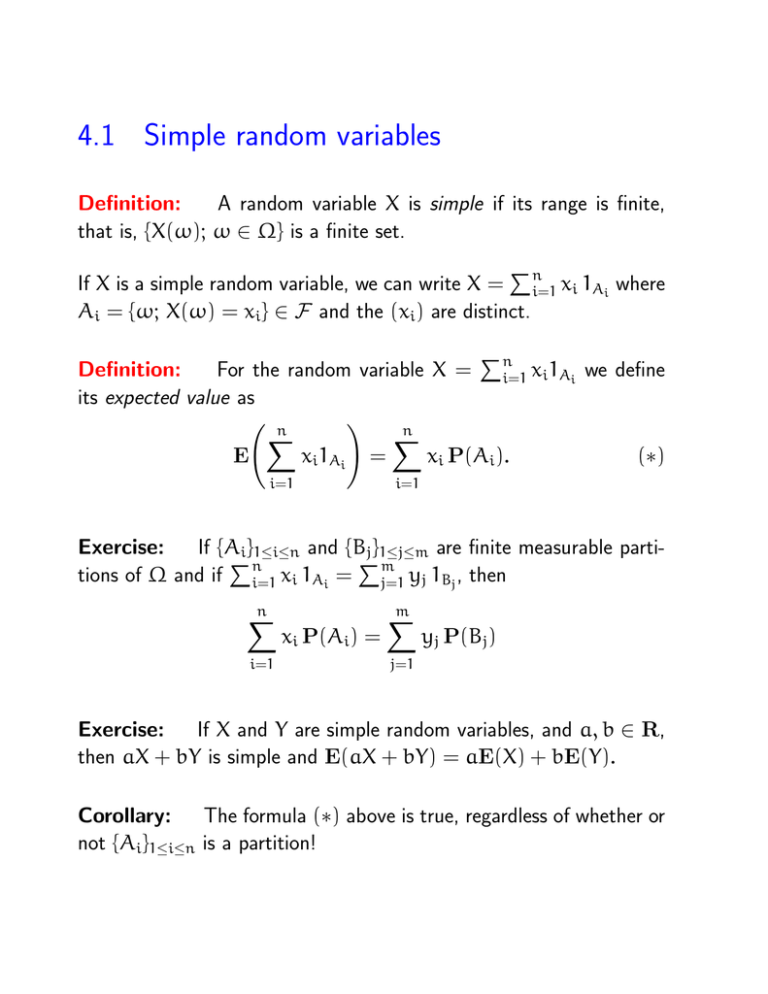
Definition:
A random variable X is simple if its range is finite,
that is, {X(ω); ω ∈ Ω} is a finite set.
P
If X is a simple random variable, we can write X = ni=1 xi 1Ai where
Ai = {ω; X(ω) = xi} ∈ F and the (xi) are distinct.
Pn
Definition:
For the random variable X = i=1 xi1Ai we define
its expected value as
!
n
n
X
X
E
xi1Ai =
xi P(Ai).
(∗)
i=1
i=1
Exercise:
If {Ai}1≤i≤n and {Bj}1≤j≤m are finite measurable partiP
P
tions of Ω and if ni=1 xi 1Ai = m
j=1 yj 1Bj , then
n
X
i=1
xi P(Ai) =
m
X
yj P(Bj)
j=1
Exercise:
If X and Y are simple random variables, and a, b ∈ R,
then aX + bY is simple and E(aX + bY) = aE(X) + bE(Y).
Corollary: The formula (∗) above is true, regardless of whether or
not {Ai}1≤i≤n is a partition!
On the probability space (Ωn, B(Ωn), Pn) of binary sequences of
length n, define the random variable X, where X(a) counts the number
of “ones” in the sequence a.
For example, when n = 7 we have X(1, 0, 0, 1, 0, 0, 1) = 3.
In general, the possible values of the random variable X are {0, 1, . . . , n}
P
so that X = nj=0 j 1(X=j).
We could also write X =
Pn
k=1 1(ak =1) .
Definition:
We write Y ≤ X if Y(ω) ≤ X(ω) for all ω ∈ Ω.
Exercise:
If Z ≥ 0, then E(Z) ≥ 0. Therefore, if Y ≤ X, then
E(Y) ≤ E(X).
Exercise:
Proposition:
Since −|X| ≤ X ≤ |X|, we have |E(X)| ≤ E(|X|).
If X is a simple random variable, then
E(X) = sup{E(Y); Y simple, Y ≤ X}.
4.2 General non-negative random variables
Definition:
If X is a non-negative random variable, define
E(X) := sup {E(Y); Y simple, Y ≤ X} ∈ [0, +∞].
Example: On ((0, 1), B, λ) the Lebesgue measure space, define
X(ω) = 1/ω2 for ω ∈ (0, 1).
For N ≥ 1, YN := N2 1(0,1/N) is a simple random variable that satisfies YN ≤ X. But E(YN) = N2 λ(0, 1/N) = N2/N = N, so
supN E(YN) = +∞ and hence E(X) = +∞.
Exercise:
If X, Z are non-negative random variables with X ≤ Z,
then E(X) ≤ E(Z).
Definition:
For random variables X1 ≤ X2 ≤ · · · with Xn(ω) →
X(ω) as n → ∞, then X is a random variable. In this case, we
say that the sequence (Xn) converges monotonically to X and write
{Xn} % X.
Proposition:
(The Monotone Convergence Theorem)
Suppose that (Xn) are non-negative random variables with {Xn} % X.
Then limn→∞ E(Xn) = E(X).
Proposition:
For any non-negative random variable X, there is a
sequence of non-negative simple random variables with {Xn} % X.
For x ≥ 0, define Ψn(x) = min(n, b2nxc/2n). Then Ψn takes finitely
many values, Ψn(x) ≥ 0 and {Ψn(x)} % x as n → ∞.
The sequence Xn := Ψn(X) does the trick!
Proposition:
If X, Y ≥ 0 and a, b ≥ 0, then
E(aX + bY) = aE(X) + bE(Y).
Proposition:
For non-negative random variables X1, X2, . . .
!
∞
∞
X
X
E(Xn).
E
Xn =
n=1
n=1
Corollary: If X is a non-negative random variable, then E(bXc) =
P∞
k=1 P(X ≥ k).
4.3 Arbitrary random variables
For any random variable, X = X+ − X− where X+ = max(X, 0) and
X− = max(−X, 0). We define the expected value of X by

E(X+) − E(X−)



+∞
E(X) =
−∞



undefined
Exercise:
if
if
if
if
E(X+) < ∞,
E(X+) = ∞,
E(X+) < ∞,
E(X+) = ∞,
E(X−) < ∞
E(X−) < ∞
E(X−) = ∞
E(X−) = ∞
If X, Y have well-defined means and X ≤ Y, then
E(X) ≤ E(Y).
Exercise:
If X, Y have finite means and a, b ∈ R, then
E(aX + bY) = aE(X) + bE(Y).
Exercise:
E(|X|) = E(X+) + E(X−).
Product measure
Given two probability spaces (Ω1, F1, P1) and (Ω2, F2, P2) we want
to define the product probability space.
The sample space Ω is the Cartesian product
Ω1 × Ω2 = {(ω1, ω2); ω1 ∈ Ω1 and ω2 ∈ Ω2}.
Define a family of subsets of this space by
J = {A × B; A ∈ F1 and B ∈ F2},
and define the product σ-field to be F1 × F2 = σ(J ).
For sets in J we define
P(A × B) = P1(A) P2(B).
Exercise:
J is a semialgebra and P(∅) = 0 and P(Ω) = 1.