NUMERICAL METHODS: Euler, Matlab, and Differential Systems
Many of the systems we study, both linear and nonlinear, are described by differential
equations. In general, the solution of these differential equations is quite difficult. Even for
those that can be solved in analytic form the solutions themselves can be difficult to interpret.
To assist in our solution of these equations we will use a variety of techniques (numerical
solution, visualization of slope fields, phase plots, etc.) for which computers are quite helpful.
Before we use computational methods we had better understand what we (and later the
computer) are doing.
The derivative
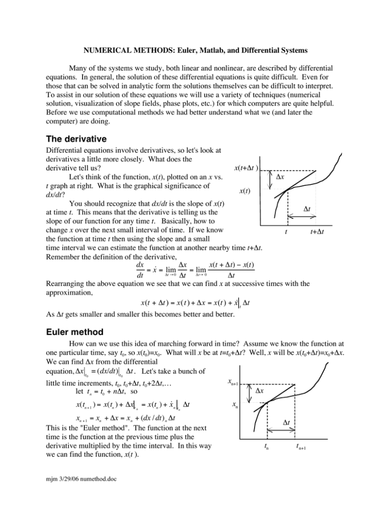
Differential equations involve derivatives, so let's look at
derivatives a little more closely. What does the
x(t+!t )
derivative tell us?
!x
Let's think of the function, x(t), plotted on an x vs.
t graph at right. What is the graphical significance of
x(t)
dx/dt?
You should recognize that dx/dt is the slope of x(t)
!t
at time t. This means that the derivative is telling us the
slope of our function for any time t. Basically, how to
change x over the next small interval of time. If we know
t
t+!t
the function at time t then using the slope and a small
time interval we can estimate the function at another nearby time t+Δt.
Remember the definition of the derivative,
dx
!x
x(t + !t) # x(t)
= x˙ = lim
= lim
!t " 0 !t
!t" 0
dt
!t
Rearranging the above equation we see that we can find x at successive times with the
approximation,
x(t + !t ) = x(t ) + !x = x(t ) + x˙ t !t
As Δt gets smaller and smaller this becomes better and better.
Euler method
How can we use this idea of marching forward in time? Assume we know the function at
one particular time, say t0, so x(t0)=x0. What will x be at t=t0+Δt? Well, x will be x(t0+Δt)=x0+Δx.
We can find Δx from the differential
equation, "x t = (dx/dt) t "t . Let's take a bunch of
0
0
xn+1
little time increments, t0, t0+Δt, t0+2Δt,…
!x
let t n = t0 + n!t, so
!
x(tn + 1 ) = x(tn ) + !x t n = x(tn ) + x˙ n tn !t
xn + 1 = xn + !x = x n + (dx / dt) n !t
This is the "Euler method". The function at the next
time is the function at the previous time plus the
derivative multiplied by the time interval. In this way
we can find the function, x(t ).
mjm 3/29/06 numethod.doc
xn
!t
tn
t n+1
Nonlinear Dynamical Systems Lab
Page 2 of 6
Numerical Methods
Euler method by hand
These methods will be easiest to think about with a specific problem in mind.
dx
Specific problem: Given the differential equation
= x˙ = ! x with x(0) = 1 ,
dt
find x(t) on the time interval 0 ! t ! 1 , in particular x(1).
Analytic solution
You may have seen this equation before and recognize the solution. If not, that's OK.
What does the differential equation tell us? The function, x(t), which satisfies the equation is
such that taking the derivative of the function with respect to time, dx/dt, gives the function itself
multiplied by -1. Can you think of any function that is basically its own derivative?
The answer is x(t)= e-t =exp(-t). So x(1)exact=0.36788.
Big step size
To get a feel for how this will go, let's try to solve our particular problem by hand using a
graphical/numerical technique. We will start at t0=0 and move forward until we are at t=1,
finding x along the way.
Starting with a time interval Δt = 1, make a table as follows and also plot the points (t,x)
(x is vertical and t is horizontal) on a sheet of graph paper as you proceed. You should have
(t0,x0), (t1,x1), …Now connect successive pairs of points with a straight line.
n
0
1
Δt
1
tn = t 0 + n!t
0
1
xn=xn-1 +Δx
1
0
(dx/dt)n=-xn
-1
Δx=(dx/dt)n Δt
-1
Smaller step size
Make another table with step size Δt = 0.5 and plot the points as you proceed.
n
0
1
2
Δt
0.5
0.5
0.5
tn = t n!1 + "t
0
0.5
1
xn=xn-1 +Δx
1
0.5
0.25
(dx/dt)n=-xn
-1
-0.5
Δx=(dx/dt)n Δt
-0.5
-0.25
Even smaller step size
Do the same thing but with a step size of Δt = 0.2. Again, make a table and a plot.
NOTE:
Items with a diamond symbol "♦" should be included as part of your lab report.
♦ Table and plot for step size of Δt = 0.2.
Question: These results do not agree with the exact answer, how could we do better?
Nonlinear Dynamical Systems Lab
Page 3 of 6
Numerical Methods
Euler method by machine
Matlab
Doing all these calculations by hand is quite tedious. Let's write a program that specifies
the differential equation, the initial conditions, the final time, and the step size. We'll let the
computer do Euler's method and then we can just list or plot the solution. Below is a program
written for the Matlab programming environment that does what we want. We'll look at the
program and then you'll program it.
% myeuler.m (name, date)
% Euler method for differential equation
clear
% initial, final, step size info
ti=0;
xi=1;
tf=1;
dt=input('enter step size: ');
% let user choose step size
% set up the variables
N=(tf-ti)/dt;
% determine number of steps
x=zeros(N+1,1);
% initialize an x vector with zeros
t=zeros(N+1,1);
% initialize a t vector with zeros
x(1)=xi;
% set first elements to starting value
t(1)=ti;
% march forward for N steps
for i=2:N+1;
dxdt=-x(i-1);
% our differential equation
dx= dxdt*dt;
% change in x
x(i)=x(i-1)+dx;
% new value of x, Euler
t(i)=t(i-1)+dt;
% new value of t, Euler
end
% output the results
t,x
% list t, x
% plot the results
figure
% makes plot the top window
plot(t,x,'ko',t,x,'k-')
% plot x vs. t, circles at points, lines too
xlabel('t')
% label the axes
ylabel('x')
title('xdot=-x by Euler method')
% title
text(0.7,0.8,['dt= ',num2str(dt) ] )
% indicate step size
text(0.7,0.7,['x(1)= ',num2str(x(N+1)) ] )
% indicate value at t=1
•
•
•
•
•
Anything after "%" is ignored by the computer, these are comments for the programmer.
The program initializes some variables and sets up vectors for storing the results.
The "for" loop is what lets us move forward in time using the Euler method.
Our specific differential equation is in the line that specifies "dxdt".
The last several lines give the output in graphical form.
Nonlinear Dynamical Systems Lab
Page 4 of 6
Numerical Methods
Enter and run this program yourself
NOTE: a) In what follows "click" means to position the mouse pointer over the specified item
and click the mouse button. b) Menu choices are indicated as File/New/M-file, which means
click on "File", move down to "New", move to "M-file" and click.
•
click on the Matlab program icon, the program will start and this should appear:
This version is for educational classroom use only.
To get started, type one of these: helpwin, helpdesk, or demo.
For product information, visit www.mathworks.com.
»
This is the "command window" and ">>" is the command line prompt where you can enter
commands. However, before we can run our program we need to enter it.
•
•
•
•
•
select File/New/M-file
an editing window should appear and a blinking cursor should be on line 1
now type in the program as shown above, change "name" to yours and "date" to today
when done, select File/Save and Execute ... type in the name of your program "myeuler.m",
save it in your folder
click somewhere back in the "command window", a blinking cursor will appear next to ">>"
your program should have run and will ask you for the step size,
enter step size: 1 <return>
A figure should appear
that looks like the one at
the right.
0.9
0.8
dt= 1
0.7
x(1)= 0
0.6
x
Record x(1).
Compare this with the
exact value
xexact(1)=exp(-1)
=0.36788.
xdot=-x by Euler method
1
0.5
0.4
0.3
0.2
0.1
0
0
0.1
0.2
0.3
0.4
0.5
t
0.6
0.7
0.8
0.9
1
Nonlinear Dynamical Systems Lab
Page 5 of 6
Numerical Methods
Euler method with smaller step size
Now run your program again and use a smaller step size, say 0.5, again write down x(1).
Repeat for step size 0.2. Displaying the values of t and x on the screen takes a while for lots of
steps. In your program change the line "t,x" to "% t,x" to prevent output. Repeat for step sizes of
0.1, 0.01, 0.001, 0.0001, each time writing down x(1).
♦ Print out your figure for step sizes 0.1 and 0.0001 (click in the figure window, select
File/Print)
Make a table to summarize your results. Include a column where you compare the numerical
result with the known result as a percent difference
x(1)numerical ! x(1)exact
percent difference =
"100
x(1)exact
step size
x(1)_numerical
x(1)_exact
% difference
1
0
0.36788
100
0.5
0.36788
0.2
0.36788
0.1
0.36788
0.01
0.36788
0.001
0.36788
0.0001
0.36788
♦ Table of percent difference like that above.
♦ What do you notice about the percent difference as the step size decreases? Is there an
obvious relationship between the decrease in percent difference and the decrease in step size?
This is a general feature of the Euler method; in most cases, if you decrease the step size
the percent difference between your numerical result and the "correct" result decreases in a linear
fashion. There are more sophisticated methods that give good results without requiring very
small step sizes.
Differential Systems
We have a program called Differential Systems with the Euler method built in, along with
some nice plotting routines. Differential Systems will be used regularly throughout the quarter so
it is important to understand its features. Let's solve the same differential equation again using it.
Almost everything about the program can be adjusted, but for most items the default settings are
reasonable.
•
•
•
Click on Differential Systems.
the program will start and show a figure with a set of axes, and two boxes, one in the
upper right and the other in the lower part of the screen.
Select Apple/Scalar Equations (Apple is in very upper left corner)
a set of axes will appear
Select Plot/Equation Definition…
a box for inputting the differential equation, in the "dx/dt=" box, type "-x",
Nonlinear Dynamical Systems Lab
Page 6 of 6
Numerical Methods
Click "Process Equation"
Select Methods/Euler
Select Plot/Fixed Step Parameters…, for Step Size type in "1", click "OK"
Select Plot/Plot Style…, choose "Interpolation Kind: linear", choose "Direction:
increasing t", "OK"
• In the box labeled "View: x vs t", enter the initial conditions, t=0, x=1. Click "Plot".
The solution to the differential equation for a step size of 1 should appear. Notice the similarity
to your Matlab solution.
•
•
•
•
Changing step size
• So the next few steps are easier to see, let's adjust the plotting region. Select Screen/Plot
Bounds…, type in -0.1 and 1.1 for the t limits (horizontal axis), and -0.1 and 1.1 for x limits
(vertical axis).
• Erase the curve we already have by selecting Screen/Erase Curves.
• Click "Plot" again. The curve from before should reappear.
• Change the step size (Plot/Fixed Step Parameters…) to 0.5, 0.1, 0.01 and take a look. The
results for the different step sizes should all appear on the same graph. You should see that
the solution depends on the step size.
♦ Print out this plot of the various solutions.
• Let's find the function at the time t=1. Move the mouse over the plot region and some
crosshairs will appear. Move the crosshairs to time t=1 and onto the various curves and read
off the value of x for t=1. (You might not get exactly t=1, maybe t=0.995 or close.)
More to Differential Systems
Up to this point we have used Differential Systems to mimic what we did with Matlab. It is
much more powerful and has many convenient features.
• Erase the existing curves, select Screen/Erase Curves.
• Click when the cross hairs are in the plotting region. A solution for that starting condition
(t0,x0) appears.
• Click somewhere else. This is a solution for this set of starting conditions.
• Select Plot/Field Marks. A slope field should appear.
Recall that the derivative tells us about the slope of the function. For our problem dx/dt=-x, the
slope depends on x. Notice that for any value of x (along a horizontal line) the slope is the same.
For given initial conditions the solution is such that it is everywhere tangent to the slope.
By now you have some sense of what is happening with the numerical solutions. Also, you
should be starting to gain some familiarity with Differential Systems.
♦ Describe in your own words how the Euler method works.
dx
♦ Consider another problem:
= x˙ = !0.2 x with x(0) = 5 , for 0<t<10. Solve this by
dt
modifying your Matlab program. You do not need to do different step sizes. Just use a step size
small enough to give results accurate to three significant figures. Also, solve it using Differential
Systems, showing the slope field (try Δt =0.1).