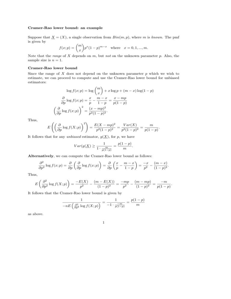
Cramer-Rao lower bound: an example
Suppose that X = (X), a single observation from Bin(m, p), where m is known. The pmf
is given by
m x
f (x; p) =
p (1 − p)m−x where x = 0, 1, ..., m.
x
Note that the range of X depends on m, but not on the unknown parameter p. Also, the
sample size is n = 1.
Cramer-Rao lower bound
Since the range of X does not depend on the unknown parameter p which we wish to
estimate, we can proceed to compute and use the Cramer-Rao lower bound for unbiased
estimators:
m
log f (x; p) = log
+ x log p + (m − x) log(1 − p)
x
∂
x m−x
x − mp
log f (x; p) = −
=
∂p
p
1−p
p(1 − p)
2
∂
(x − mp)2
log f (x; p) = 2
.
∂p
p (1 − p)2
Thus,
E
2 !
∂
E(X − mp)2
V ar(X)
m
log f (X; p)
= 2
= 2
=
.
2
2
∂p
p (1 − p)
p (1 − p)
p(1 − p)
It follows that for any unbiased estimator, g(X), for p, we have
V ar(g(X) ≥
1
1·
m
p(1−p)
=
p(1 − p)
.
m
Alternatively, we can compute the Cramer-Rao lower bound as follows:
∂2
∂
∂
∂ x m−x
−x (m − x)
log f (x; p) =
log f (x; p) =
−
= 2 −
.
2
∂p
∂p ∂p
∂p p
1−p
p
(1 − p)2
Thus,
E
∂2
−E(X) (m − E(X))
−mp (m − mp)
−m
log f (X; p) =
−
=
−
=
.
2
2
2
2
2
∂p
p
(1 − p)
p
(1 − p)
p(1 − p)
It follows that the Cramer-Rao lower bound is given by
1
−nE
∂2
∂p2
=
−1 ·
log f (X; p)
as above.
1
1
−m
p(1−p)
=
p(1 − p)
m
Handout #1
Comparing estimators
Consider the estimator g1 (X) =
X
m.
E(g1 (X)) =
E(X)
mp
=
=p
m
m
so g1 (X) is an unbiased estimator of p. Is it the most efficient unbiased estimator for p?
To answer this question, we compute the variance of g1 and compare it to the Cramer-Rao
lower bound which we calculated above.
V ar(g1 (X)) = V ar(
X
V ar(X)
mp(1 − p)
p(1 − p)
)=
=
=
.
2
2
m
m
m
m
Since V ar(g1 ) equals the Cramer-Rao lower bound, we can conclude that g1 (X) is the
most efficient unbiased estimator for p.
Now consider the estimator g2 (X) =
E(g2 (X)) =
X+1
m+2 .
E(X) + 1
mp + 1
=
6= p (except when p = 1/2).
m+2
m+2
So g2 is a biased estimator with
bias(g2 ) = E(g2 (X)) − p =
mp + 1
1 − 2p
−p=
.
m+2
m+2
To compare the performance of g2 with the performance of g1 , we must first compute the
mean square error of g2 :
V ar(g2 (X)) = V ar(
V ar(X + 1)
mp(1 − p)
X +1
)=
=
.
2
m+2
(m + 2)
(m + 2)2
Thus,
M SE(g2 ) = V ar(g2 )+(bias(g2 ))2 =
1
mp(1 − p) (1 − 2p)2
+
=
(1+(m−4)p−(m−4)p2 ).
2
2
(m + 2)
(m + 2)
(m + 2)2
We can compare the (relative) efficiency of g1 and g2 by comparing the graphs of M SE(g1 )
(which is just the variance of g1 ) and M SE(g2 ) as functions of p.
Exercise: Fix m = 10 and sketch the graphs of M SE(g1 ) and M SE(g2 ) as functions of
p. Also, determine the values of p for which g2 is more efficient than g1 .
2