THE REGRESSION MODEL IN MATRIX FORM
$%$%$%$%$%$%$%$%$%$%$%$%$%$%$%$%$%$%$%
We will consider the linear regression model in matrix form.
For simple linear regression, meaning one predictor, the model is
Yi = β0 + β1 xi + εi
for i = 1, 2, 3, …, n
This model includes the assumption that the εi ’s are a sample from a population with mean zero
and standard deviation σ. In most cases we also assume that this population is normally
distributed.
The multiple linear regression model is
Yi = β0 + β1 xi1 + β2 xi2 + β3 xi3 + … + βK xiK + εi
for i = 1, 2, 3, …, n
This model includes the assumption about the εi ’s stated just above.
This requires building up our symbols into vectors. Thus
Y
n ×1
⎛ Y1 ⎞
⎜Y ⎟
⎜ 2⎟
= ⎜ Y3 ⎟
⎜ ⎟
⎜# ⎟
⎜Y ⎟
⎝ n⎠
captures the entire dependent variable in a single symbol. The “n × 1” part of the notation is
just a shape reminder. These get dropped once the context is clear.
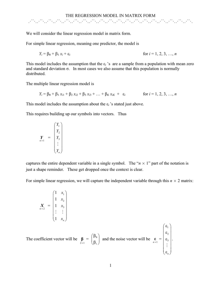
For simple linear regression, we will capture the independent variable through this n × 2 matrix:
⎛1
⎜1
⎜
X = ⎜1
n×2
⎜
⎜#
⎜1
⎝
x1 ⎞
x2 ⎟⎟
x3 ⎟
⎟
# ⎟
xn ⎟⎠
⎛ ε1 ⎞
⎜ε ⎟
⎜ 2⎟
⎛ β0 ⎞
The coefficient vector will be β = ⎜ ⎟ and the noise vector will be ε = ⎜ ε3 ⎟ .
n ×1
2 ×1
⎜ ⎟
⎝ β1 ⎠
⎜# ⎟
⎜ε ⎟
⎝ n⎠
1
THE REGRESSION MODEL IN MATRIX FORM
$%$%$%$%$%$%$%$%$%$%$%$%$%$%$%$%$%$%$%
The simple linear regression model is written then as Y
n ×1
=
X β + ε .
n × 2 2 ×1
n ×1
The product part, meaning X β , is found through the usual rule for matrix multiplication as
n × 2 2 ×1
X β
n × 2 2 ×1
⎛1
⎜1
⎜
= ⎜1
⎜
⎜#
⎜1
⎝
x1 ⎞
x2 ⎟⎟
x3 ⎟
⎟
#⎟
xn ⎟⎠
⎛ β0
⎜
⎜ β0
⎛ β0 ⎞
⎜ ⎟ = ⎜ β0
⎜
⎝ β1 ⎠
⎜
⎜β
⎝ 0
+ β1 x1 ⎞
⎟
+ β1 x2 ⎟
+ β1 x3 ⎟
⎟
#
⎟
+ β1 xn ⎟⎠
We usually write the model without the shape reminders as Y = X β + ε.
notation for
⎛ β0 + β1
⎛ Y1 ⎞
⎜
⎜Y ⎟
⎜ β0 + β1
⎜ 2⎟
⎜ Y3 ⎟ = ⎜ β0 + β1
⎜
⎜ ⎟
⎜#
⎜# ⎟
⎜Y ⎟
⎜β + β
1
⎝ n⎠
⎝ 0
This is a shorthand
x1 + ε1 ⎞
⎟
x2 + ε2 ⎟
x3 + ε3 ⎟
⎟
⎟
xn + εn ⎟⎠
It is helpful that the multiple regression story with K ≥ 2 predictors leads to the same model
expression Y = X β + ε (just with different shapes). As a notational convenience, let
p = K + 1. In the multiple regression case, we have
X
n× p
⎛1
⎜1
⎜
⎜1
⎜
1
= ⎜
⎜1
⎜
⎜1
⎜#
⎜⎜
⎝1
x11
x21
x31
x41
x51
x61
#
xn 1
x12 " x1K ⎞
x22 " x2 K ⎟⎟
x32 " x3 K ⎟
⎟
x42 " x4 K ⎟
x52 " x5 K ⎟
⎟
x62 " x6 K ⎟
# % # ⎟
⎟
xn 2 " xnK ⎟⎠
⎛ β0 ⎞
⎜ ⎟
⎜ β1 ⎟
⎜β ⎟
β = ⎜ 2⎟
p ×1
⎜ β3 ⎟
⎜# ⎟
⎜⎜ ⎟⎟
⎝ βK ⎠
and
The detail shown here is to suggest that X is a tall, skinny matrix. We formally require n ≥ p.
n
In most applications, n is much, much larger than p. The ratio
is often in the hundreds.
p
2
THE REGRESSION MODEL IN MATRIX FORM
$%$%$%$%$%$%$%$%$%$%$%$%$%$%$%$%$%$%$%
n
is as small as 5, we will worry that we don’t have enough
p
data (reflected in n) to estimate the number of parameters in β (reflected in p).
If it happens that
The multiple regression model is now Y
n ×1
⎛ β0
⎛ Y1 ⎞
⎜
⎜Y ⎟
⎜ β0
⎜ 2⎟
⎜ Y3 ⎟ = ⎜ β0
⎜
⎜ ⎟
⎜
⎜# ⎟
⎜Y ⎟
⎜β
⎝ n⎠
⎝ 0
=
X β + ε
n × p p ×1
n ×1
, and this is a shorthand for
+ β1 x11 + β2 x12 + β3 x13 + " + β K x1K + ε1 ⎞
⎟
+ β1 x21 + β2 x22 + β3 x23 + " + β K x2 K + ε 2 ⎟
+ β1 x31 + β 2 x32 + β3 x33 + " + β K x3K + ε3 ⎟
⎟
#
⎟
+ β1 xn1 + β2 xn 2 + β3 xn 3 + " + β K xnK + ε n ⎟⎠
The model form Y = X β + ε is thus completely general.
The assumptions on the noise terms can be written as E ε = 0 and Var ε = σ2 I. The I here is
the n × n identity matrix. That is,
⎛1
⎜0
⎜
I = ⎜0
⎜
⎜#
⎜0
⎝
"
"
"
%
0 0 "
0
1
0
#
0
0
1
#
0⎞
0 ⎟⎟
0⎟
⎟
#⎟
1 ⎟⎠
⎛ σ2
⎜
⎜0
The variance assumption can be written as Var ε = ⎜ 0
⎜
⎜ #
⎜0
⎝
2
this expressed as Cov( εi , εj ) = σ δij , where
⎧1
δij = ⎨
⎩0
if i = j
if i ≠ j
3
0
σ2
0
#
0
0 " 0⎞
⎟
0 " 0⎟
σ2 " 0 ⎟ . You may see
⎟
# % # ⎟
0 " σ2 ⎟⎠
THE REGRESSION MODEL IN MATRIX FORM
$%$%$%$%$%$%$%$%$%$%$%$%$%$%$%$%$%$%$%
We will call b as the estimate for unknown parameter vector β .
You will also find the notation β̂ as the estimate.
Once we get b , we can compute the fitted vector Yˆ = X b . This fitted value represents an
ex-post guess at the expected value of Y.
The estimate b is found so that the fitted vector Yˆ is close to the actual data vector Y.
Closeness is defined in the least squares sense, meaning that we want to minimize the
criterion Q, where
∑ (Y
n
Q =
i =1
i
−
( X b )i
th
entry
)
2
This can be done by differentiating this quantity p = K + 1 times, once with respect to b0, once
with respect to b1, ….., and once with respect to bK . This is routine in simple regression
(K = 1), and it’s possible with a lot of messy work in general.
It happens that Q is the squared length of the vector difference Y − Xb . This means that we
can write
Q = (Y − Xb )′ (Y − Xb )
1× n
n ×1
This represents Q as a 1 × 1 matrix, and so we can think of Q as an ordinary number.
There are several ways to find the b that minimizes Q. The simple solution we’ll show here
(alas) requires knowing the answer and working backward.
Define the matrix H
n×n
=
X
n× p
( X′ X )
p×n n× p
−1
X ′ . We will call H as the “hat matrix,” and it has
p×n
some important uses. There are several technical comments about H :
(1)
(2)
Finding H requires the ability to get
( X′ X )
p×n n× p
−1
. This matrix inversion is
possible if and only if X has full rank p. Things get very interesting when X
almost has full rank p ; that’s a longer story for another time.
The matrix H is idempotent. The defining condition for idempotence is this:
The matrix C is idempotent ⇔ C C = C .
Only square matrices can be idempotent.
Since H is square (It’s n × n.), it can be checked for idempotence. You will
indeed find that H H = H .
4
THE REGRESSION MODEL IN MATRIX FORM
$%$%$%$%$%$%$%$%$%$%$%$%$%$%$%$%$%$%$%
(3)
The ith diagonal entry, that in position (i, i), will be identified for later use as the
ith leverage value. The notation is usually hi , but you’ll also see hii .
Now write Y in the form H Y + (I – H) Y .
Now let’s develop Q. This will require using the fact that H is symmetric, meaning H ′ = H .
This will also require using the transpose of a matrix product. Specifically, the property will be
( X b )′ = b′ X ′ .
Q = (Y − Xb )′ (Y − Xb )
=
( {H Y + ( I − H ) Y } −
=
( {H Y
Xb
)′ ( {H Y + ( I − H )Y } −
Xb
)
− Xb} + ( I − H ) Y )′ ( {H Y − Xb} + ( I − H )Y )
=
{H Y
− Xb}′ {H Y − Xb}
+
{H Y
− Xb}′ ( I − H ) Y
+
( ( I − H )Y )′ {H Y
+
( ( I − H )Y )′ ( I − H )Y
− Xb}
The second and third summands above are zero, as a consequence of
−1
( I − H ) X = X − H X = X − X ( X ′ X ) X ′ X = X − X = 0.
=
{H Y
− Xb}′ {H Y − Xb} +
( ( I − H )Y )′ ( I − H )Y
If this is to be minimized over choices of b, then the minimization can only be done with regard
to the first summand {H Y − Xb}′ {H Y − Xb} . It is possible to make the vector
H Y − Xb equal to 0 by selecting b = ( X ′ X ) X ′ Y . This is very easy to see, as
-1
H = X (X′ X ) X′.
-1
This b = ( X ′ X ) X ′ Y is known as the least squares estimate of β.
-1
5
THE REGRESSION MODEL IN MATRIX FORM
$%$%$%$%$%$%$%$%$%$%$%$%$%$%$%$%$%$%$%
⎛b ⎞
For the simple linear regression case K = 1, the estimate b = ⎜ 0 ⎟ and be found with relative
⎝ b1 ⎠
n
n
S
ease. The slope estimate is b1 = xy , where Sxy = ∑ ( xi − x ) (Yi − Y ) = ∑ xiYi − n x Y
S xx
i =1
i =1
n
and where Sxx =
∑( x − x )
i =1
i
2
n
=
∑x
i =1
2
i
− n (x) .
2
For the multiple regression case K ≥ 2, the calculation involves the inversion of the p × p
matrix X′ X. This task is best left to computer software.
There is a computational trick, called “mean-centering,” that converts the problem to a
simpler one of inverting a K × K matrix.
The matrix notation will allow the proof of two very helpful facts:
*
E b = β . This means that b is an unbiased estimate of β . This is a good
thing, but there are circumstances in which biased estimates will work a little bit
better.
*
Var b = σ2 ( X ′ X ) . This identifies the variances and covariances of the
estimated coefficients. It’s critical to note that the separate entries of b are not
statistically independent.
−1
6