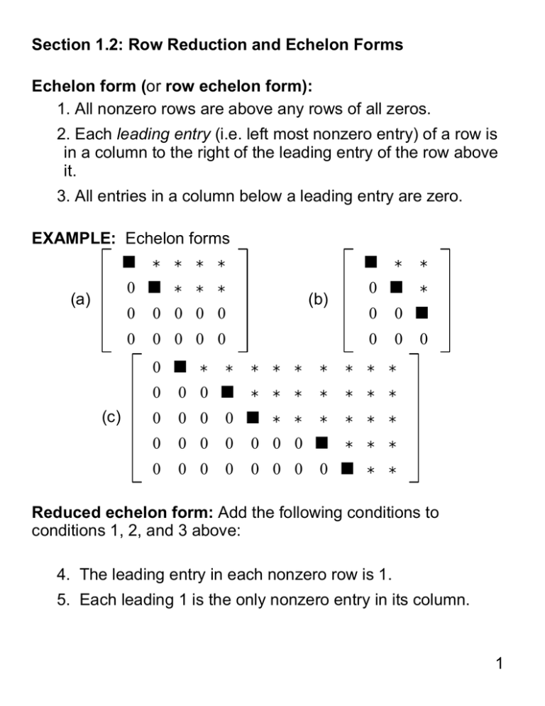
Section 1.2: Row Reduction and Echelon Forms
Echelon form (or row echelon form):
1. All nonzero rows are above any rows of all zeros.
2. Each leading entry (i.e. left most nonzero entry) of a row is
in a column to the right of the leading entry of the row above
it.
3. All entries in a column below a leading entry are zero.
EXAMPLE: Echelon forms
■ ∗ ∗ ∗ ∗
■
0 ■ ∗ ∗ ∗
(a)
0
0 0 0 0
0
0 0 0 0
0 ■ ∗
(c)
(b)
∗
∗
0 ■
∗
0
0 ■
0
0
∗
∗ ∗ ∗
∗
∗ ∗ ∗
0
0 0 ■
∗ ∗ ∗
∗
∗ ∗ ∗
0
0 0
0 ■ ∗ ∗
∗
∗ ∗ ∗
0
0 0
0
0 0 0 ■
∗ ∗ ∗
0
0 0
0
0 0 0
0
0 ■ ∗ ∗
Reduced echelon form: Add the following conditions to
conditions 1, 2, and 3 above:
4. The leading entry in each nonzero row is 1.
5. Each leading 1 is the only nonzero entry in its column.
1
EXAMPLE (continued):
Reduced echelon form :
0 1 ∗ 0 0 ∗ ∗ 0 0 ∗ ∗
0 0 0 1 0 ∗ ∗ 0 0 ∗ ∗
0 0 0 0 1 ∗ ∗ 0 0 ∗ ∗
0 0 0 0 0 0 0 1 0 ∗ ∗
0 0 0 0 0 0 0 0 1 ∗ ∗
Theorem 1 (Uniqueness of The Reduced Echelon Form):
Each matrix is row-equivalent to one and only one
reduced echelon matrix.
2
Important Terms:
●
pivot position: a position of a leading entry in an echelon
form of the matrix.
●
pivot: a nonzero number that either is used in a pivot
position to create 0’s or is changed into a leading 1, which in
turn is used to create 0’s.
●
pivot column: a column that contains a pivot position.
(See the Glossary at the back of the textbook.)
3
EXAMPLE: Row reduce to echelon form and locate the pivot
columns.
0 −3 −6
4
9
−1 −2 −1
3
1
−2 −3
3 −1
1
0
5 −9 −7
4
Solution
pivot
↙
1
4
5 −9 −7
−1 −2 −1
3
−2 −3
3 −1
0
0 −3 −6
4
1
9
↑
pivot column
1
4
5
−9
−7
0
2
4
−6
−6
0
5 10 −15 −15
0 −3 −6
4
9
Possible Pivots:
4
1 4 5 −9 −7
0 2 4 −6 −6
0 0 0
0
0
0 0 0 −5
0
1 4 5 −9 −7
∼
Original Matrix:
pivot columns:
0 2 4 −6 −6
0 0 0 −5
0
0 0 0
0
0
0 −3 −6
4
9
−1 −2 −1
3
1
−2 −3
3 −1
0
5 −9 −7
1
4
↑
↑
↑
1 2
4
Note: There is no more than one pivot in any row. There is no
more than one pivot in any column.
5
EXAMPLE: Row reduce to echelon form and then to reduced
echelon form:
3 −6
0
3 −7
6 4 −5
8 −5 8
9
3 −9 12 −9 6 15
Solution:
0
3 −6
3 −7
6 4 −5
8 −5 8
3 −9 12 −9 6 15
∼
9
3 −7
3 −9 12 −9 6 15
0
8 −5 8
3 −6
9
6 4 −5
3 −9 12 −9 6 15
∼
0
2 −4
4 2 −6
0
3 −6
6 4 −5
Cover the top row and look at the remaining two rows for the
left-most nonzero column.
3 −9 12 −9 6 15
0
2 −4
4 2 −6
0
3 −6
6 4 −5
3 −9 12 −9 6 15
∼
0
1 −2
2 1 −3
0
3 −6
6 4 −5
3 −9 12 −9 6 15
∼
0
1 −2
2 1 −3
0
0
0 1
0
(echelon form)
4
6
Final step to create the reduced echelon form:
Beginning with the rightmost leading entry, and working upwards
to the left, create zeros above each leading entry and scale rows
to transform each leading entry into 1.
3 −9 12 −9 0 −9
0
1 −2
2 0 −7
0
0
0 1
0
3 0 −6 9 0 −72
∼
4
0 1 −2 2 0
0 0
0 0 1
−7
4
1 0 −2 3 0 −24
∼
0 1 −2 2 0
0 0
0 0 1
−7
4
7
SOLUTIONS OF LINEAR SYSTEMS
●
basic variable: any variable that corresponds to a pivot
column in the augmented matrix of a system.
● free variable: all nonbasic variables.
EXAMPLE:
1 6 0
3 0 0
0 0 1 −8 0 5
0 0 0
0 1 7
x 1 +6x 2
+3x 4
=0
x 3 −8x 4
=5
x5 = 7
pivot columns:
basic variables:
free variables:
8
Final Step in Solving a Consistent Linear System: After the
augmented matrix is in reduced echelon form and the system is
written down as a set of equations:
Solve each equation for the basic variable in terms of the free
variables (if any) in the equation.
EXAMPLE:
x 1 = −6x 2 − 3x 4
x 1 +6x 2
+3x 4
=0
x 2 is free
x 3 −8x 4
=5
x 3 = 5 + 8x 4
x5 = 7
x 4 is free
x5 = 7
(general solution)
The general solution of the system provides a parametric
description of the solution set. (The free variables act as
parameters.) The above system has infinitely many solutions.
Why?
Warning: Use only the reduced echelon form to solve a
system.
9
Existence and Uniqueness Questions
EXAMPLE:
−6x 3 +6x 4 +4x 5 = −5
3x 2
3x 1 −7x 2
+8x 3 −5x 4 +8x 5
=9
3x 1 −9x 2 +12x 3 −9x 4 +6x 5 = 15
In an earlier example, we obtained the echelon form:
3 −9 12 −9 6 15
0
2 −4
4 2 −6
0
0
0 1
0
4
x 5 = 4 
No equation of the form 0 = c, where c ≠ 0, so the system is
consistent.
Free variables: x 3 and x 4
Consistent system
 infinitely many solutions.
with free variables
10
EXAMPLE:
3x 1 +4x 2 = −3
2x 1 +5x 2 =
5
−2x 1 −3x 2 =
1
→
3 4 −3
∼
0 1
3
0 0
0

Consistent system,
no free variables
3
4 −3
2
5
5
−2 −3
1
3x 1 + 4x 2 = −3
x2 = 3
 unique solution.
11
Theorem 2 (Existence and Uniqueness Theorem)
1. A linear system is consistent if and only if the rightmost
column of the augmented matrix is not a pivot column, i.e., if
and only if an echelon form of the augmented matrix has no
row of the form
0 . . . 0 b (where b is nonzero).
2. If a linear system is consistent, then the solution contains
either
(i) a unique solution (when there are no free variables) or
(ii) infinitely many solutions (when there is at least one free
variable).
Using Row Reduction to Solve Linear Systems
1. Write the augmented matrix of the system.
2. Use the row reduction algorithm to obtain an equivalent
augmented matrix in echelon form. Decide whether the system is
consistent. If not, stop; otherwise go to the next step.
3. Continue row reduction to obtain the reduced echelon form.
4. Write the system of equations corresponding to the matrix
obtained in step 3.
5. State the solution by expressing each basic variable in terms of
the free variables and declare the free variables.
12
EXAMPLE:
a) What is the largest possible number of pivots a 4 × 6 matrix can
have? Why?
b) What is the largest possible number of pivots a 6 × 4 matrix can
have? Why?
c) How many solutions does a consistent linear system of 3
equations and 4 unknowns have? Why?
d) Suppose the coefficient matrix corresponding to a linear
system is 4 × 6 and has 3 pivot columns. How many pivot
columns does the augmented matrix have if the linear system is
inconsistent?
13