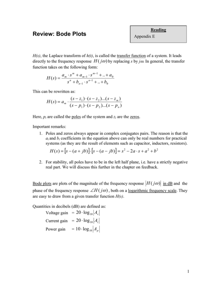
Review: Bode Plots
Reading
Appendix E
H(s), the Laplace transform of h(t), is called the transfer function of a system. It leads
directly to the frequency response H ( jω ) by replacing s by jω. In general, the transfer
function takes on the following form:
H (s) =
a m ⋅ s m + a m −1 ⋅ s m −1 + .. + a 0
s n + bn −1 ⋅ s n −1 + .. + b0
This can be rewritten as:
H (s) = am ⋅
( s − z1 ) ⋅ ( s − z 2 )...( s − z m )
( s − p1 ) ⋅ ( s − p 2 )...( s − p n )
Here, pi are called the poles of the system and zi are the zeros.
Important remarks:
1. Poles and zeros always appear in complex conjugates pairs. The reason is that the
ai and bi coefficients in the equation above can only be real numbers for practical
systems (as they are the result of elements such as capacitor, inductors, resistors).
H ( s ) = [s − ( a + jb ) ]⋅ [s − ( a − jb ) ] = s 2 − 2 a ⋅ s + a 2 + b 2
2. For stability, all poles have to be in the left half plane, i.e. have a strictly negative
real part. We will discuss this further in the chapter on feedback.
Bode plots are plots of the magnitude of the frequency response H ( jω ) in dB and the
phase of the frequency response ∠ H ( jω ) , both on a logarithmic frequency scale. They
are easy to draw from a given transfer function H(s).
Quantities in decibels (dB) are defined as:
Voltage gain = 20 ⋅ log 10 Av
Current gain = 20 ⋅ log 10 Ai
Power gain
= 10 ⋅ log 10 A p
1
To draw the Bode plots based on a transfer function, it is easiest to split it first up in a
concatenation of first and second order functions H1(s), H2(s), H3(s), etc.
H (s) = am ⋅
H 1 ( s ) ⋅ H 2 ( s ) ⋅ ...
H 3 ( s ) ⋅ H 4 ( s ) ⋅ ...
Magnitude:
H (s) = am ⋅
H 1 ( s ) ⋅ H 2 ( s ) ⋅ ...
H 3 ( s ) ⋅ H 4 ( s ) ⋅ ...
20 ⋅ log10 H ( s ) = 20 ⋅ log10 am + 20 ⋅ log10 H 1 ( s ) + ... − 20 ⋅ log10 H 3 ( s ) − ...
Phase:
∠H ( s ) = ∠am + ∠H 1 ( s ) + ∠H 2 ( s ) + ... − ∠H 3 ( s ) − ∠H 4 ( s ) − ...
First order sections:
(a)
H (s) = s
→
H ( jω ) = jω
20 ⋅ log H ( jω ) = 20 ⋅ log(ω )
∠ H ( jω ) =
π
2
|H(jω)| (dB)
∠H(jω)
π/2
0
100
101
102 ω (log scale)
0
100
101
102
ω (log scale)
2
(b)
H (s) = 1 +
s
= 1+τ ⋅ s
a
H ( jω ) = 1 +
→
jω
= 1 + jωτ
a
2
⎛ω ⎞
2
20 ⋅ log H ( jω ) = 20 ⋅ log 1 + ⎜ ⎟ = 20 ⋅ log 1 + (ωτ )
⎝a⎠
∠H ( jω ) = tan −1 (ωτ )
small ω:
20 ⋅ log H ( jω ) ≈ 20 ⋅ log 1 = 0
large ω:
20 ⋅ log H ( jω ) ≈ 20 ⋅ log
decade: ω · 10
octave: ω · 2
ω = |a| = 1/|τ|:
ω
a
(assume a > 0)
= 20 ⋅ log ωτ = 20 ⋅ log ω + 20 ⋅ log τ
→
→
20 dB
6 dB
20 ⋅ log H ( jω ) ≈ 20 ⋅ log 2 = 3 dB
|H(jω)| (dB)
small ω:
∠H ( jω ) ≈ tan −1 (0) = 0
large ω:
∠H ( jω ) ≈ tan −1 (∞ ) =
ω = |a| = 1/|τ|:
∠H ( jω ) ≈ tan −1 (1) =
π
2
π
4
3
∠H(jω)
5.7°
90°
45°
Actual
0°
0.1·|a|
5.7°
|a|
10·|a|
ω (log scale)
For a concatenation of functions, just add the respective Bode plots.
There is also an easy way to generate the Bode plot for the magnitude directly, or use it to
check if you added everything up correctly. Just follow the following procedure:
1.
At low frequencies (ω → 0), set s = 0. This will result in something of the form
H ( s ) = a ⋅ s n where n could by positive or negative
H ( jω ) = a ⋅ ( jω ) = a ⋅ ω n
n
20 ⋅ log H ( jω ) = n ⋅ 20 ⋅ log ω + 20 ⋅ log a
20 ⋅ log H ( jω ) = 0
⇔
ω=a
→ (20·n) dB/decade
−1 / n
This means that at low frequencies, the plot has an asymptote with a slope of 20n
decibels per decade. It is shifted such that it would intersect the 0 dB axis at
ω=a
−1 / n
.
2.
At each pole, add -20 dB/decade.
At each zero, add +20 dB/decade.
3.
Check at high frequencies (ω → ∞), s → ∞. Again you will get something of the
form
H (s) = a ⋅ s n
4
Additional Remarks
For the part of the curve that is sloping up,
we made the approximation
H ( jω ) = 1 +
|H(jω)| (dB)
ω
jω
jω
≈
=
a
a
a
20 ⋅ log H ( jω ) ≈ 20 ⋅ log
ω
a
= 20 ⋅ log ω + 20 ⋅ log
ω · 10
decade:
1
a
→
→
|H| · 10
|H| increases by 20 dB
This means that on the curve with a slope of 20 dB/decade, if we consider
a frequency that is 10 times higher (a decade), the magnitude goes up by
20 dB on the decibel scale. Equivalently, in real units, the magnitude is 10
times higher.
in general ∀y:
ω·y
→
|H| · y
On the curve with a slope of 20 dB/decade, if we consider a frequency that
is y times higher, the magnitude in real units goes up by y as well.
For example:
|H(jω)| (dB)
80
-20 dB/decade
A
0
10 kHz
40 kHz
ω1
What is the value of A, both in real units and in dB?
What is the value of ω1?
5