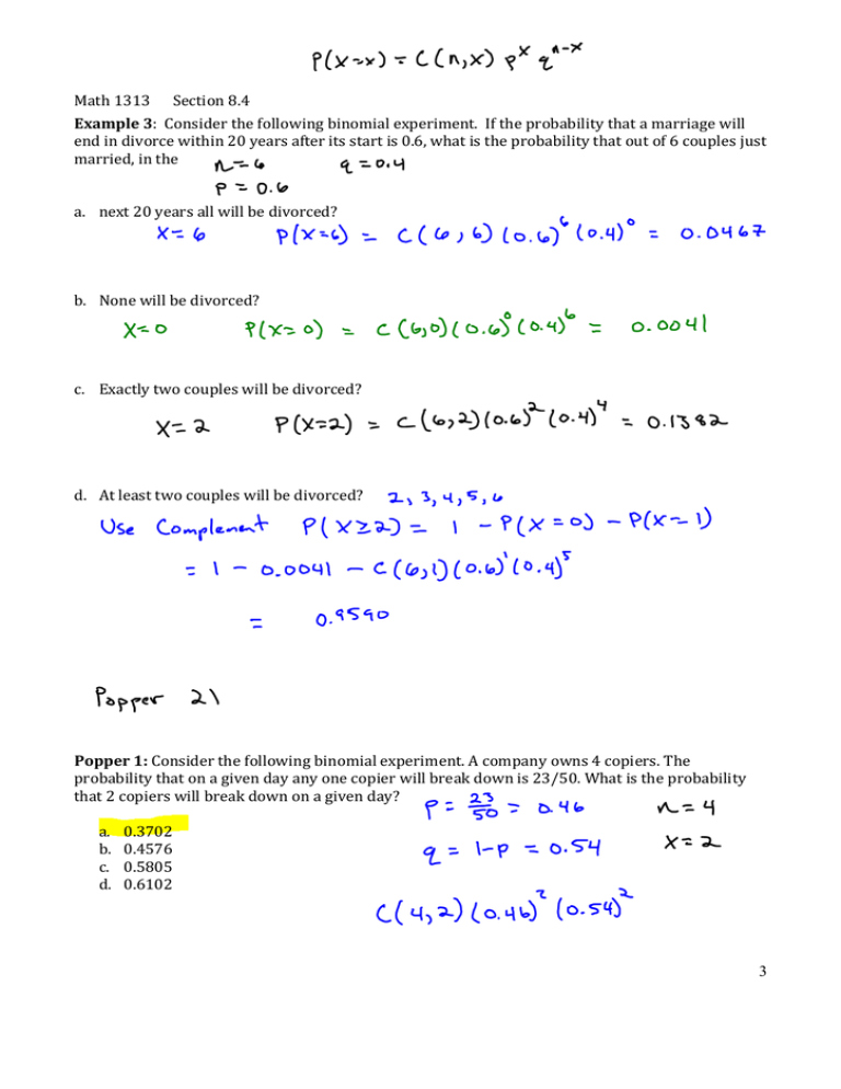
Math 1313
Section 8.4
Example 3: Consider the following binomial experiment. If the probability that a marriage will
end in divorce within 20 years after its start is 0.6, what is the probability that out of 6 couples just
married, in the
a. next 20 years all will be divorced?
b. None will be divorced?
c. Exactly two couples will be divorced?
d. At least two couples will be divorced?
Popper 1: Consider the following binomial experiment. A company owns 4 copiers. The
probability that on a given day any one copier will break down is 23/50. What is the probability
that 2 copiers will break down on a given day?
a.
b.
c.
d.
0.3702
0.4576
0.5805
0.6102
3
Math 1313
Section 8.4
Example 4: A baseball pitcher gives up a hit on the average of once every fifth pitch. If nine
pitches are thrown, what is the probability that
a. Exactly three of them result in a hit?
b. None of them result in a hit?
Mean, Variance and Standard Deviation of a Random Variable
If X is a binomial random variable associated with a binomial experiment consisting of n trials with
probability of success p, and probability of failure q, then the mean E(X), variance and standard
deviation of X are given by applying the following formulas:
ߤ = ‫ ܧ‬ሺܺሻ = ݊‫݌‬
ܸܽ‫ݎ‬ሺܺ ሻ = ݊‫ݍ݌‬
ߪ = ඥܸܽ‫ݎ‬ሺܺሻ = ඥ݊‫ݍ݌‬
Example 5: The probability of a person contracting influenza on exposure is 62%. In the
binomial experiment for a family of 12 that has been exposed, what is the:
a. mean?
b. standard deviation?
c. variance?
4
Math 1313
Section 8.4
Popper 2: A company owns 4 copiers. The probability that on a given day any one copier will
break down is 0.64. What is the probability that at least 2 copiers will break down on a given day?
a.
b.
c.
d.
0.8638
0.6960
0.5398
0.5806
Popper 3: Consider the following binomial experiment. The probability that a fuse produced by a
certain company will be defective is 11/50. If 500 fuses are produced each day, how many can we
expect to find each day that are defective?
a.
b.
c.
d.
107
110
112
113
5
Math 1313 Section 8.5
Section 8.5: The Normal Distribution
A random variable that may take on infinitely many values is called a continuous random
variable.
The probability distribution associated with this type of random variable is called a continuous
probability distribution.
A continuous probability distribution is defined by a function f called the probability density
function. The function has domain equal to those values the continuous random variable
assumes.
The probability density function has the following properties:
1. f(x) >0 for all values of x.
2. The area between the curve and the x axis is 1.
The probability that the random variable X associated with a given probability density function
assumes a value in an interval a < x < b is given by the area of the region between the graph of f
and the x-axis from x = a to x = b.
Here is a picture:
This value is ܲሺܽ ൏ ܺ ൏ ܾሻ
Note: ܲሺܽ ൏ ܺ ൏ ܾሻ ൌ ܲሺܽ ൏ ܺ ൏ ܾሻ ൌ ܲሺܽ ൏ ܺ ൏ ܾሻ ൌ ܲሺܽ ൏ ܺ ൏ ܾሻ, since the area under one
point is 0.
1
Math 1313
Section 8.5
Normal Distributions.
For these types of distributions:
1. The graph is a bell-shaped curve.
2. ߤ and ߪ each have the same meaning (mean and standard deviation)
3. ߤ determines the location of the center of the curve.
4. ߪ determines the sharpness or flatness of the curve.
Also, the normal curve has the following characteristics:
1. The curve has peak at x = ߤ.
2. The curve is symmetric with respect to the vertical line x = ߤ.
3. The curve always lies above the x-axis but approaches the x-axis as x extends indefinitely in
either direction.
4. The area under the curve is 1.
5. For any normal curve, 68.27% of the area under the curve lies within 1 standard deviation of
the mean (i.e. between ߤ − ߪ and ߤ + ߪ), 95.45% of the area lies within 2 standard deviations of
the mean, and 99.73% of the area lies within 3 standard deviations of the mean.
Since any normal curve can be transformed into any other normal curve we will study, from here
on, the Standard Normal Curve.
The Standard Normal Curve has ߤ =0 and ߪ =1.
The corresponding distribution and random variable are called the Standard Normal
Distribution and the Standard Normal Random Variable, respectively.
The Standard Normal Variable will commonly be denoted Z.
2
Math 1313
Section 8.5
The area of the region under the standard normal curve to the left of some value z, i.e. P(Z < z)
or P(Z ≤ z), is calculated for us in Table II, Appendex B on pg. 1177.
Example 1: Let Z be the standard normal variable. By first making a sketch of the appropriate
region under the standard normal curve, find the values of:
a. P(Z < -1.91)
b. P(Z < 0.44)
c. P(Z > 0.5)
d. P(Z > 2.56)
e. P(-1.65 < Z < 2.02)
f. P(1 < Z < 2.47)
3
Math 1313
Section 8.5
Example 2: Let Z be the standard normal variable. Find the value of z if z satisfies:
a. P(Z < z) = 0.9495
b. P(Z > z) = 0.9115
c. P(Z < -z) = 0.6950
d. P(-z < Z < z) = 0.7888
e. P(-z < Z < z) = 0.8444
4