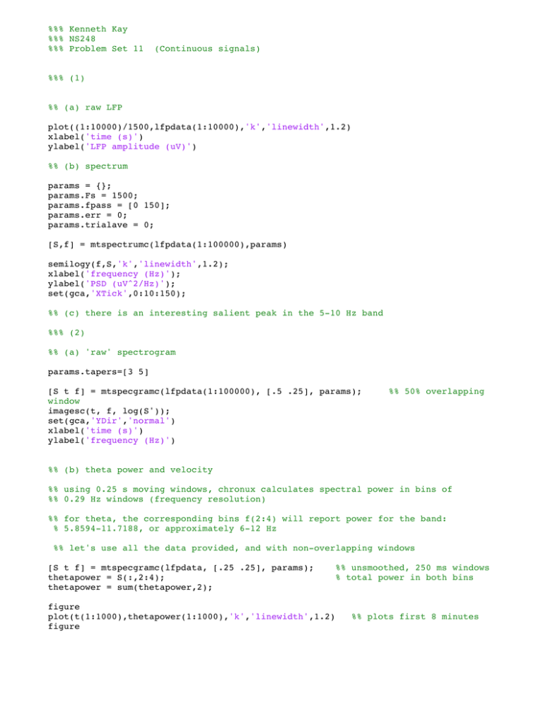
%%% Kenneth Kay
%%% NS248
%%% Problem Set 11
(Continuous signals)
%%% (1)
%% (a) raw LFP
plot((1:10000)/1500,lfpdata(1:10000),'k','linewidth',1.2)
xlabel('time (s)')
ylabel('LFP amplitude (uV)')
%% (b) spectrum
params = {};
params.Fs = 1500;
params.fpass = [0 150];
params.err = 0;
params.trialave = 0;
[S,f] = mtspectrumc(lfpdata(1:100000),params)
semilogy(f,S,'k','linewidth',1.2);
xlabel('frequency (Hz)');
ylabel('PSD (uV^2/Hz)');
set(gca,'XTick',0:10:150);
%% (c) there is an interesting salient peak in the 5-10 Hz band
%%% (2)
%% (a) 'raw' spectrogram
params.tapers=[3 5]
[S t f] = mtspecgramc(lfpdata(1:100000), [.5 .25], params);
window
imagesc(t, f, log(S'));
set(gca,'YDir','normal')
xlabel('time (s)')
ylabel('frequency (Hz)')
%% 50% overlapping
%% (b) theta power and velocity
%% using 0.25 s moving windows, chronux calculates spectral power in bins of
%% 0.29 Hz windows (frequency resolution)
%% for theta, the corresponding bins f(2:4) will report power for the band:
% 5.8594-11.7188, or approximately 6-12 Hz
%% let's use all the data provided, and with non-overlapping windows
[S t f] = mtspecgramc(lfpdata, [.25 .25], params);
thetapower = S(:,2:4);
thetapower = sum(thetapower,2);
figure
plot(t(1:1000),thetapower(1:1000),'k','linewidth',1.2)
figure
%% unsmoothed, 250 ms windows
% total power in both bins
%% plots first 8 minutes
plot(t,thetapower,'k','linewidth',1.2)
%% plots all 15 minutes
%% for velocity, we want to bin postimes the same way as the chronux spectrogram
%% does the LFP -- that is, in 250 ms windows
%% specifically, we'll take the mean of speed in 250 ms windows
windowsize_sec = 0.25 ;
postimes_Fs = 1/(postimes(2)-postimes(1));
windowsize_possamples = windowsize_sec*postimes_Fs;
firstindex=1;
speed_in_windows = nan(1,length(t)-20);
%% truncate last 20 windows
for i=1:length(speed_in_windows)
velocity =
mean(abs(speed(floor(firstindex):floor((firstindex+windowsize_possamples)))));
speed_in_windows(i)=velocity;
firstindex = firstindex+windowsize_possamples;
end
figure
plotyy((1:1000)/4,thetapower(1:1000),(1:1000)/4,speed_in_windows(1:1000))
xlabel('time (s)')
ylabel('theta power (uV^2)')
scatter(thetapower(1:(end-20)),speed_in_windows,'k','.');
xlabel('theta power (uV^2)')
ylabel('mean velocity')
figure
scatter(thetapower(1:(end-20)),speed_in_windows,'k','.');
xlabel('theta power (uV^2)')
ylabel('mean velocity')
set(gca,'xscale','log')
% linear scale
% log scale
[R,P,RLO,RUP]=corrcoef(thetapower(1:(end-20)),speed_in_windows);
relationship
%% assumes linear
% yields R=-0.0869, p=1.79e-07 -- there seems to be a highly significant
% weak negative correlation
%%%% (3)
%% (a) You can readily specify the amount of attenuation or amplification
%% at the various stopbands and passbands.
%% (b) In general, higher levels of attenuation/amplification tend to increase the
%% order of the filter.
%% (c) Tighter bandpass filters require higher order filters.
%%%% (4)
%% (a)
%% matlab 'filter'
filtered_data = [];
filtered_data = filter(thetafilter.tf.num,thetafilter.tf.den,lfpdata);
plot((1:4500)/1500,filtered_data(1:4500),'r','linewidth',1.2);
xlabel('time (s)')
ylabel('LFP (uV)')
hold on
plot((1:4500)/1500,lfpdata(1:4500),'k','linewidth',1);
%% poor match -- the filter has shifted the phase of the theta
%% frequency component, resulting in huge mismatch from the
%% original signal (which has lots of theta)
%% the beginning of trace is very noticeably mismatched
%% matlab 'filtfilt'
figure
filtered_data = [];
filtered_data = filtfilt(thetafilter.tf.num,thetafilter.tf.den,lfpdata);
plot((1:4500)/1500,filtered_data(1:4500),'r','linewidth',1.2);
xlabel('time (s)')
ylabel('LFP (uV)')
hold on
plot((1:4500)/1500,lfpdata(1:4500),'k','linewidth',1);
%%
the phases now appear to match
%%%% (5)
%% (a)
hilbert_data = hilbert(filtered_data);
hilbert_envelope = abs(hilbert_data);
figure
hold on
plot((1:4500)/1500,hilbert_envelope(1:4500),'b','linewidth',1.2);
plot((1:4500)/1500,-hilbert_envelope(1:4500),'b','linewidth',1.2);
plot((1:4500)/1500,filtered_data(1:4500),'k','linewidth',1);
xlabel('time (s)')
ylabel('LFP (uV)')
%% amplitude looks correct
%% (b)
figure
hold on
plotyy((3500:4500)/1500,angle(hilbert_data(3500:4500)), ...
(3500:4500)/1500,filtered_data(3500:4500));
xlabel('time (s)')
ylabel('LFP (uV)')
%% phase looks correct
%% (c) phase histogram
%% preliminary function findindex, since spiketimes values aren't corresponding
%% exactly to lfptimes... :
% % function output = findindex(v,value);
% %
% % % this function returns the index of vector v closest to value
%
%
%
%
%
%
%
%
%
%
%
%
%
%
%
%
%
%
%
%
%
%
%
%
%
%
%
%
%
%
%
%
%
%
%
%
%
%
%
%
%
%
% v is assumed to be sorted in increasing order
% rounds upwards by default
greater_than = v>=value;
less_than = v<=value;
test=greater_than.*less_than;
if sum(test) == 1
%% value is already in v
output=find(test);
elseif prod(double(less_than ~= greater_than))==1 %% value is between two elements
greaterindex = find(greater_than,1);
lessindex = greaterindex-1;
if abs(value-v(lessindex)) < abs(v(greaterindex)-value)
output = lessindex;
else
output = greaterindex;
end
else
disp('value not contained within vector');
end
end
hilbert_phases = angle(hilbert_data);
spike_phases = nan(1,length(spiketimes));
%% initialize
for s=1:length(spiketimes)
spike_phases(s) = hilbert_phases(findindex(lfptimes,spiketimes(s)));
end
hist(spike_phases,20)
xlabel('phase (rads)')
ylabel('# spikes')
%% (d) spike-triggered LFP averages
windowsize = 1;
windowsize_samp = 1500;
eegwindows = nan(length(spiketimes),windowsize_samp*2+1);
for s=1:length(spiketimes)
centerindex = findindex(lfptimes,spiketimes(s));
eegwindows(s,:) = lfpdata((centerindexwindowsize_samp):(centerindex+windowsize_samp));
end
STA = mean(eegwindows,1);
plot((-1500:1500),STA,'k','linewidth',1.5);
xlabel('time (s)')
ylabel('LFP amplitude (uV)')
%% spike-triggered average indicates an increase in theta is
%% strongly associated with spikes
%% (e) phase precession
%% we already have spike_phases, now do the same for position:
spike_positions = nan(1,length(spiketimes));
%% initialize
for s=10:length(spiketimes)
spike_positions(s) = pos(findindex(postimes,spiketimes(s)));
end
scatter(spike_positions,spike_phases,'.','k')
%% there appears to be a weak negative correlation between position and
%% phase at several positions (one near 0 position, and one near 110 cm)
%% (f) directional effect
%% conveniently the speed data is actually velocity, thus we can use the
%% sign of the speed data to distinguish trial direction
spikes_LR = []
spikes_RL = []
;
;
% let positions occupy 1st column, and phases the 2nd
for s=10:length(spiketimes)
dir = sign(speed(findindex(postimes,spiketimes(s))));
if dir==1
%% LR
spikes_LR = [spikes_LR ; [pos(findindex(postimes,spiketimes(s))) ...
hilbert_phases(findindex(lfptimes,spiketimes(s)))] ];
else
%% RL
spikes_RL = [spikes_RL ; [pos(findindex(postimes,spiketimes(s))) ...
hilbert_phases(findindex(lfptimes,spiketimes(s)))] ];
end
end
figure
scatter(spikes_LR(:,1),spikes_LR(:,2),'.','k')
title('right to left trials')
xlabel('linear position (cm)')
ylabel('theta phase (rads)')
figure
scatter(spikes_RL(:,1),spikes_RL(:,2),'.','k')
title('left to left trials')
xlabel('linear position (cm)')
ylabel('theta phase (rads)')