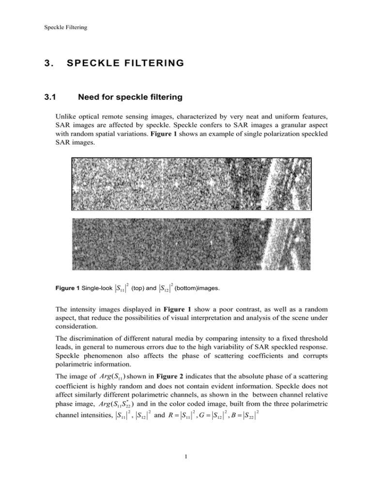
Speckle Filtering
3.
SPECKLE FILTERING
3.1
Need for speckle filtering
Unlike optical remote sensing images, characterized by very neat and uniform features,
SAR images are affected by speckle. Speckle confers to SAR images a granular aspect
with random spatial variations. Figure 1 shows an example of single polarization speckled
SAR images.
Figure 1 Single-look S11
2
2
(top) and S12 (bottom)images.
The intensity images displayed in Figure 1 show a poor contrast, as well as a random
aspect, that reduce the possibilities of visual interpretation and analysis of the scene under
consideration.
The discrimination of different natural media by comparing intensity to a fixed threshold
leads, in general to numerous errors due to the high variability of SAR speckled response.
Speckle phenomenon also affects the phase of scattering coefficients and corrupts
polarimetric information.
The image of Arg ( S11 ) shown in Figure 2 indicates that the absolute phase of a scattering
coefficient is highly random and does not contain evident information. Speckle does not
affect similarly different polarimetric channels, as shown in the between channel relative
*
phase image, Arg ( S11 S 22
) and in the color coded image, built from the three polarimetric
2
channel intensities, S 11 , S 12
2
and R = S 11 , G = S 12 , B = S 22
2
1
2
2
Speckle Filtering
Figure
2
Arg ( S11 )
(top)
R = S11 , G = S12 , B = S 22
2
2
and
2
*
Arg ( S11 S 22
)
(middle)
images.
Color
coded
image
(bottom).
Speckle corrupts polarimetric observables (phase and intensity) in an important way. Specific
procedures have to be used to retrieve relevant polarimetric information and to reduce the
randomness of the acquired signals.
3.2
Simple speckle model
3.2.1
Single-polarization multiplicative speckle model
Speckle confers a random aspect to SAR images, but may not be considered as a simple noise.
It is, in fact, tightly related to the SAR measurement principle.
Synthesized SAR data may be considered as the result of the integration of a scene coherent
response within each resolution cell, resulting from the convolution of the SAR impulse
response with the coherent contribution of each elementary scatterer, as illustrated in Figure
3. As the number of contributing scatterers, within a resolution cell, tends to be large (it is the
case for common resolution SAR measurements), the resulting integrated response is random
in phase and amplitude and is shown to follow, over homogeneous areas, a Normal
distribution.
2
Speckle Filtering
Im
Ei
E tot = ∑ E i
i
E1
Re
Figure 3 Principle of coherent integration.
A speckled response is usually represented under the form of a simple product model
y = x.n
(1)
Where y represents a complex speckled scattering coefficient, x the original unspeckled
scattering coefficient and n the multiplicative speckle contribution.
The speckle term, n is composed of independent real and imaginary parts, following both real
centered Normal distribution N C (0, 1 / 2) .
The corresponding speckled intensity, Y , is
Y = yy ∗ = xx ∗ nn∗
⇒ Y = X nn ∗
(2)
Over homogeneous areas, X is considered to be constant and the speckled intensity follows
an exponential probability density function
−1
p (Y ) = X e
−
Y
X
(3)
Its first two moments are given by
E (Y ) = X E (nn ∗ ) = X
Var (Y ) = X 2 Var (nn ∗ ) = X 2
3.2.2
(4)
Polarimetric multiplicative speckle model
This speckle model may be extended to the polarimetric case by considering that polarimetric
channels are affected by independent multiplicative speckle components :
3
Speckle Filtering
⎡ S11 ⎤ ⎡ x11
⎢S ⎥ = ⎢
⎢ 12 ⎥ ⎢
⎢⎣ S 22 ⎥⎦ ⎢⎣
x12
⎡ S11 2 ⎤ ⎡ X (n n ∗ ) ⎤
11
11 11
⎢
2⎥
⎢
∗ ⎥
⎢ S12 ⎥ = ⎢ X 12 (n12 n12 ) ⎥
⎢ S 2 ⎥ ⎢ X (n n ∗ )⎥
⎣⎢ 22 ⎦⎥ ⎣ 22 22 22 ⎦
⎤ ⎡ n11 ⎤
⎥⎢n ⎥ ⇒
⎥ ⎢ 12 ⎥
x22 ⎥⎦ ⎢⎣n22 ⎥⎦
(5)
One may note that the multiplicative assumption is in general not valid to model speckled
correlation terms.
3.3
Principle of scalar speckle filtering
3.3.1
Incoherent averaging
As presented in the former paragraph, a speckled intensity, Y , may be considered as a
random variable whose mean value equals the unspeckled intensity, X , but affected by a
large variance due to speckle.
The principle of speckle filtering consists of reducing the variance of Y in order to improve
the estimate of its mean.
The sample mean, Y , is defined as the empirical average of L independent realizations of a
speckled intensity as follows
Y =
1 L
∑ Yi
L i =1
(6)
It can be shown that, over homogeneous areas, this estimate of X follows a Gamma density
function
p( Y ) =
L −1
LL X Y
Γ( L ) X
L
e
−
L Y
X
(7)
and has the following two first moments
E( Y ) = X
Var ( Y ) = X 2 / L
(8)
It is possible to observe from (8) that as the number of independent samples, L, reduces to 1
the variance of the estimate intensity increases, whereas incoherent averaging over L
independent realizations permits to reduce the variance of a speckled intensity in a significant
way.
The quantity L = var( I ) / E ( I ) 2 is called the Equivalent Number of Looks (ENL) and is a
measure of speckle importance.
4
Speckle Filtering
stdev ( Y
)
10n
4
10
9
3.5
8
3
7
2.5
6
5
2
4
1.5
3
1
2
0.5
1
0
0
0
2
4
E( Y
)
6
8
10
Figure 4 Occurrence (scattering diagram) of single-look of intensity moments over a homogeneous
areas.
The occurrence plot displayed in Figure 4 clearly shows that the standard deviation and the
mean of sampled intensities are linearly related over homogeneous areas. The slope of this
linear relation is L and equals 1 in the case of single-look data sets.
3.3.2
Boxcar and J. S. Lee filters
3.3.2.1
The boxcar filter
The boxcar filter is a direct application of the incoherent averaging described by (6) to the
case of an image.
~
Filtered intensity estimates, X i , j , are constructed by computing the sample mean over each
pixel neighborhood, defined by a sliding window of ( N w × N w ) pixels
~
X i , j = Yi , j
Nw
=
1
N w2
Nw / 2
∑
Nw / 2
∑Y
i+ p , j +q
p=− N w / 2 q=− N w / 2
(9)
where the subscripts i and j correspond to the considered pixel row and column index
respectively.
2
Figure 5 S11 filtered image using a boxcar filter.
5
Speckle Filtering
Figure 5 shows an intensity image obtained using a (7×7) boxcar filter. This image shows
enhanced contrast and lower random aspect.
As it can be seen in Figure 5, the boxcar filter is characterized by two main limitations :
-
sharp edges are generally blurred
-
point scatterers are over filtered and transformed to spread targets
Solutions to these limitations are offered by the refined Lee filter.
3.3.2.2
J.S. Lee adaptive filter
J. S. Lee's filter determines the unspeckled intensity estimate that minimizes the mean squared
error
~
X−X
2
(10)
This MMSE filter is based on a linearized speckle model leading to the following estimate
expression
~
X = Y N +k Y − Y N
(11)
w
w
(
)
where k is an adaptive filtering coefficient, based on local statistics, given by
2
2
var( X ) var Y − E ( Y )σ n
k=
=
var Y
var Y [1 + σ n2 ]
(12)
1
2
with σ n = the a priori speckle variance
L
~
Over homogeneous areas, var( X ) = 0 ⇒ k = 0 and X = Y N , whereas over point targets
w
~
and highly heterogeneous areas, k = 1⇒ X = Y and the pixel intensity remains unaffected by
the filtering procedure.
0
1
Figure 6 Examples of directional masks.
In order to reduce the sensitivity of the adaptive filtering coefficient, k , to isolated
heterogeneities, this filter uses directional masks to determine the most homogeneous part of
the sliding window where local statistics have to be estimated. This modification permits to
preserve relatively sharp edges.
6
Speckle Filtering
The Lee filter results displayed in Figure 7 demonstrate the effectiveness of this adaptive
filtering approach
2
Figure 7 S11 filtered image using a (7×7) Lee filter.
3.4
Extension to the polarimetric case
3.4.1
Second order polarimetric representations
Speckle filtering is based on incoherent averaging and requires handling statistical second
order representations. The intensity information used in the scalar case has to be extended to
the vector case when dealing with two or more polarization channels in order to take into
account the different intensities as well as the cross-correlation related information.
A simple way to build an incoherent polarimetric representation consists in vectorizing the
scattering matrix to create a target vector and computing the corresponding covariance matrix
(details on matrix incoherent representations may be found in the appendix).
[S ] ⇒ k 3L , k 3P
[
]
T
with k 3 L = S11
2 S12 S 22
1
[S11 + S 22 S11 − S 22 2S12 ]T
and k 3 P =
2
(13)
The (3×3) covariance matrix, [C3 ] , is defined as :
[C3 ] = k 3 L k 3L
†
(14)
where † represents the transpose conjugate operator. One may note that [C3 ] is not a usual
covariance matrix that would require the use of an expectation operator, but this
representation may be understood as an incoherent polarimetric form obtained from a single
realization of k 3L .
The (3×3) coherency matrix, [T3 ] , is defined as :
[T3 ] = k 3 P k 3 P
†
7
(15)
Speckle Filtering
One may note that the coherency matrix is in fact the single realization covariance matrix of
k 3P .
Covariance and coherency matrices are similar (related by a similarity transformation) and
may be used in an equivalent way
k 3 P = [ A]k 3 L
⎡
⎢
⎢
−1
†
⇒ [T3 ] = [ A][C3 ][ A] = [ A][C3 ][ A] with [ A] = ⎢
⎢
⎢⎣
3.4.2
Polarimetric boxcar and Lee's filters
3.4.2.1
Polarimetric boxcar filter
1
2
0
1
2
1
2
0
1
−
2
⎤
0⎥
⎥
1⎥
0⎥
⎥⎦
(16)
The extension of the boxcar filter to the polarimetric case is straightforward. The estimated
covariance matrix is given by
~
[C ]i , j = [C ]i , j
Nw
=
1
N w2
Nw / 2
∑
Nw / 2
∑ [C ]
p=− N w / 2 q=− N w / 2
i+ p, j+q
(17)
where the subscripts i and j correspond to the considered pixel row and column index
respectively.
3.4.2.2
J. S. Lee polarimetric filter
J. S. Lee proposed to estimate the unspeckled covariance matrix according to the following
expression
~
[C ] = [C ] + k ([C ] − [C ] )
(18)
where k remains a scalar coefficient computed from the span statistics, span = C11 + C 22 + C33 .
This approximation allows to filter polarimetric data in a fast and simple way and avoids
additional coupling (or cross-talk) between the polarimetric channels.
Figure 8 shows improved color coded images processed through the boxcar and J. S. Lee
filters.
8
Speckle Filtering
Figure 8 Color-coded, R = S11 , G = S12 , B = S 22
2
2
2
, filtered image using a (7×7) boxcar (top)
Lee's filter (bottom).
3.5
Consequences of polarimetric speckle filtering
It was seen in former paragraphs that it is necessary to reduce polarimetric variables random
aspect by speckle filtering prior to any interpretation of polarimetric information. The
incoherent averaging of [T3 ] or [C3 ] matrices has an important impact on their polarimetric
properties.
3.5.1
Interpretation loss vs. information gain
Speckle filtering may cause a loss of polarimetric information by destroying the relation
between and [T3 ] or [C3 ] matrices.
A coherency matrix is fully defined by 9 real coefficients : its three diagonal terms and three
complex correlation coefficients. In the case of a single look coherency matrix, all three
correlation coefficients have unitary modulus and one of their phase may be obtained by a
linear combination of the remaining two, leaving 5 degrees of freedom. A relative scattering
matrix [ S rel ] and single-look [T3 ] or [C3 ] matrices may be related in a unique way as shown
in the following example :
⎡C11
[C ] = ⎢⎢C12*
*
⎣⎢C13
C12
C 22
*
C 23
C13 ⎤ ⎡ C11
m12 e jφ12
⎢
C 23 ⎥⎥ = ⎢m12 e − jφ12
C 22
−
j
φ
C33 ⎦⎥ ⎢⎣ m13e 13 m23 e − j (φ13 −φ12 )
with mij = Cii C jj
9
m13 e jφ13 ⎤
⎥
m23 e j (φ13 −φ12 ) ⎥
⎥
C33
⎦
(19)
Speckle Filtering
And
⎡
[S rel ] = e − jφ [S ] = ⎢
1
C11
− jφ
⎢⎣ C 22 / 2 e 12
C 22 / 2 e − jφ12 ⎤
⎥C33 e − jφ13 ⎥⎦
(20)
The scattering mechanism may then be interpreted by comparing
[S rel ]
to canonical
examples.
After speckle filtering, this may not be true anymore. In a general case, the modulus of
correlation coefficients is inferior to one and the phase terms are linearly independent
S ij S kl*
2
≤ S ij
2
S kl
2
(
and Arg S ij S kl*
)≠
(
Arg S ij S kl*
)
(21)
In such a case, the coherency matrix is said to be distributed and cannot be related to a
coherent scattering matrix.
The correlation coefficient displayed in Figure 9 shows a varying modulus over the selected
scene, indicating that the degree of correlation might be related to the nature of the scattering
medium. The additional information contained in the cross-correlation terms will be exploited
by incoherent decomposition theorems to extract even more characteristics from polarimetric
data sets.
10
Speckle Filtering
Figure 9 Argument (top) and modulus (bottom) of
*
S11S 22
/
S11
2
S 22
2
after application of a
Lee filter.
3.5.2
Partially polarized waves and polarimetric signature
As it is demonstrated in the appendix, polarization signatures may be built indifferently from
coherent scattering matrix or incoherent Kennaugh matrix representations.
The Co-polarization polarimetric signature is given by
2
PC = E (φ ,τ ) [ S ] E (φ ,τ ) or PC = g (φ ,τ ) [ K ] g (φ ,τ )
t
t
(22)
Let us assume that the Kenaugh matrix [K ] results from the incoherent averaging of N
single-look matrices [ K i ] . The Co-polarization polarimetric signature of [K ] may then be
expressed as
PC = g (φ ,τ ) [ K ] g (φ ,τ ) = g (φ ,τ ) [ K ] g (φ ,τ ) = g (φ ,τ ) g r (φ ,τ )
t
t
t
(23)
where g r (φ ,τ ) stands for the average reflected Stokes vector and may be formulated as
g r (φ ,τ ) =
1 N
1 N
[
K
]
g
(
φ
,
τ
)
=
∑ i
∑ g (φ ,τ )
N i =1
N i =1 ri
(24)
Knowing that each reflected Stokes vector may be written as a function of the corresponding
Jones vector components, that is
[
g ri = E ri1 + E ri 2
2
2
E ri1 − E ri 2
2
(
2ℜ E ri1 E ri* 2
2
)
(
− 2ℑ E ri1 E ri* 2
)]
T
(25)
The average reflected Stokes vector may be expressed as
[
g r = E r1
= [g r 0
g r1
+ Er 2
2
2
E r1
2
− Er 2
2
(
2ℜ Er1 Er*2
)
(
− 2ℑ Er1 Er*2
)]
T
gr3 ]
(26)
T
gr2
From the Cauchy-Schwarz inequality, we know that
g r20 ≥ g r21 + g r22 + g r23
(27)
Relation (27) indicates that the average polarization-dependent intensity of a wave,
g r21 + g r22 + g r23 may be inferior to its total average intensity g r20 (when the reflected Stokes
vector are not parallel).
Such waves are said to be partially polarized and may be decomposed as follows
g r = [g r 0
g r1
gr2
g r 3 ] = [(α g r 0
T
g r1
11
gr2
g r 3 ] + [(1 − α ) g r 0
T
0 0 0]
T
(28)
Speckle Filtering
Where
[(α g r 0
g r1
gr2
g r 3 ] represents
t
α 2 g r20 = g r21 + g r22 + g r23 and [(1 − α ) g r 0
(insensitive to polarization) term.
a
fully
polarized
wave,
with
0 0 0] is associated to a completely unpolarized
t
The decomposition factor
α=
g r21 + g r22 + g r23
, 0 ≤α ≤1
g r20
(29)
is called the wave degree of polarization.
The co-polarization polarimetric signature mentioned at the beginning of this paragraph can
then be rewritten as a function of the degree of polarization
⎡α g r 0 ⎤
⎢ g ⎥
t
t
PC = g (φ ,τ ) g r (φ ,τ ) = g (φ ,τ ) ⎢ r1 ⎥ + (1 − α ) g 0 g r 0
⎢ gr2 ⎥
⎥
⎢
⎣ gr3 ⎦
(30)
When the reflected Stokes vectors are not parallel, i.e. the averaged Kenaugh matrices do not
correspond by a scalar factor, α ≠ 1 and it the copular intensity is strictly superior to. In such
cases, one cannot determine co-pol nor cross-pol nulls and the polarization signature is said to
show a pedestal.
12