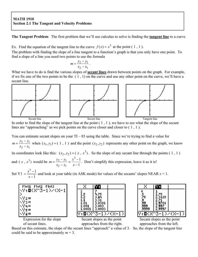
MATH 1910
Section 2.1 The Tangent and Velocity Problems
The Tangent Problem: The first problem that we’ll use calculus to solve is finding the tangent line to a curve.
Ex. Find the equation of the tangent line to the curve f ( x ) = x 3 at the point ( 1 , 1 ).
The problem with finding the slope of a line tangent to a function’s graph is that you only have one point. To
find a slope of a line you need two points to use the formula
y −y
m= 2 1 .
x2 − x1
What we have to do is find the various slopes of secant lines drawn between points on the graph. For example,
if we fix one of the two points to be the ( 1 , 1) on the curve and use any other point on the curve, we’ll have a
secant line.
Secant line
Secant line
Tangent line
In order to find the slope of the tangent line at the point ( 1 , 1 ), we have to see what the slope of the secant
lines are “approaching” as we pick points on the curve closer and closer to ( 1 , 1 ).
You can estimate secant slopes on your TI – 83 using the table. Since we’re trying to find a value for
y −y
m = 2 1 when ( x1 , y1 ) = ( 1 , 1 ) and the point ( x2 , y2 ) represents any other point on the graph, we know
x2 − x1
its coordinates look like this: ( x2 , y2 ) = ( x , x 3 ) . So the slope of any secant line through the points ( 1 , 1 )
and ( x , x 3 ) would be m =
Set Y1 =
y2 − y1 x 3 − 1
. Don’t simplify this expression, leave it as it is!
=
x2 − x1
x −1
x3 − 1
and look at your table (in ASK mode) for values of the secants’ slopes NEAR x = 1.
x −1
Expression for the slope
Secant slopes as the point
Secant slopes as the point
of secant lines.
approaches from the right.
approaches from the left.
Based on this estimate, the slope of the secant lines “approach” a value of 3. So, the slope of the tangent line
could be said to be approximately m = 3.
MATH 1910
Section 2.1 The Tangent and Velocity Problems
The equation of the tangent line to the curve at the point ( 1 , 1 ) would be y − 1 = 3( x − 1) which simplifies to
y = 3x − 2 in slope – intercept form.
The Velocity Problem: now we’ll take this notion of a curve’s tangent and apply it to velocity problems.
Ex. The position of a car is given by values in the table:
t (seconds)
s (feet)
0
0
1
10
2
32
3
70
4
119
5
178
a) Find the average velocity for the time period beginning when t = 2 and lasting for
(i) 3 sec
(ii) 2 sec
(iii) 1 sec
b) Use the graph of s as a function of t to estimate the instantaneous velocity when t = 2.
SOLUTION:
We define “average velocity” as a change in distance divided by a change in time. Simply how far did
someone drive the car in how many seconds? Starting at t = 2 , the car was a distance of 32 feet from its
starting point. From t = 2 until 3 seconds later when t = 5 , the car had driven a distance of 178 – 32 = 146 ft.
178 − 32 146
So, this makes the average velocity of the car on that time interval to be
=
= 48. 6 ft / sec.
5− 2
3
119 − 32 87
From t = 2 until 2 seconds later when t = 4 , the average velocity would be
=
= 435
. ft / sec.
4−2
2
70 − 32 38
Finally, from t = 2 until t = 3 the average velocity on this time interval would be
=
= 38 ft / sec.
3− 2
1
Our problem is, we can only use the points given to find these average velocities. One way to estimate the
instantaneous velocity of the car at t = 2 seconds is to take the average of the slopes of the secant lines before
and after t = 2 . We already know the secant slope from t = 2 to t = 3 is 38, an average velocity of 38 ft / sec.
32 − 10 22
The secant slope from t = 1to t = 2 is
=
= 22 ft / sec. So, perhaps the instantaneous velocity at
2 −1
1
t = 2 would be exactly half way between 38 ft / sec and 22 ft / sec. These numbers average out to 30 ft / sec.
The instantaneous velocity of the car is defined as the “limiting value” of these average velocities taken over
shorter and shorter time intervals that start at t = 2 seconds.
Notice the similarities in this problem and the tangent problem.
We could also get a good estimate for the instantaneous velocity by plotting a curve between the points of this
graph and estimating the slope of the tangent line at x = 2 using graphing paper and some good estimates for
values of ( x1 , y1 ) and ( x2 , y2 ) . But again, these are all estimates obtained by taking smaller and smaller
increments away from the central point t = 2.