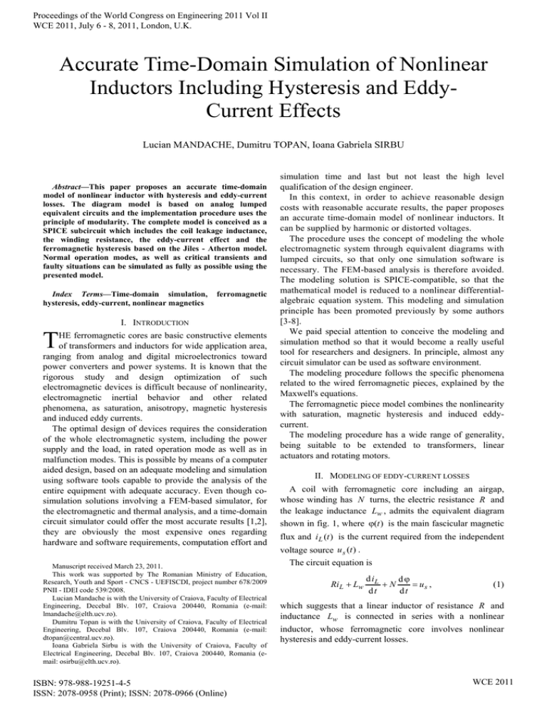
Proceedings of the World Congress on Engineering 2011 Vol II
WCE 2011, July 6 - 8, 2011, London, U.K.
Accurate Time-Domain Simulation of Nonlinear
Inductors Including Hysteresis and EddyCurrent Effects
Lucian MANDACHE, Dumitru TOPAN, Ioana Gabriela SIRBU
Abstract—This paper proposes an accurate time-domain
model of nonlinear inductor with hysteresis and eddy-current
losses. The diagram model is based on analog lumped
equivalent circuits and the implementation procedure uses the
principle of modularity. The complete model is conceived as a
SPICE subcircuit which includes the coil leakage inductance,
the winding resistance, the eddy-current effect and the
ferromagnetic hysteresis based on the Jiles - Atherton model.
Normal operation modes, as well as critical transients and
faulty situations can be simulated as fully as possible using the
presented model.
Index Terms—Time-domain simulation,
hysteresis, eddy-current, nonlinear magnetics
T
ferromagnetic
I. INTRODUCTION
HE ferromagnetic cores are basic constructive elements
of transformers and inductors for wide application area,
ranging from analog and digital microelectronics toward
power converters and power systems. It is known that the
rigorous study and design optimization of such
electromagnetic devices is difficult because of nonlinearity,
electromagnetic inertial behavior and other related
phenomena, as saturation, anisotropy, magnetic hysteresis
and induced eddy currents.
The optimal design of devices requires the consideration
of the whole electromagnetic system, including the power
supply and the load, in rated operation mode as well as in
malfunction modes. This is possible by means of a computer
aided design, based on an adequate modeling and simulation
using software tools capable to provide the analysis of the
entire equipment with adequate accuracy. Even though cosimulation solutions involving a FEM-based simulator, for
the electromagnetic and thermal analysis, and a time-domain
circuit simulator could offer the most accurate results [1,2],
they are obviously the most expensive ones regarding
hardware and software requirements, computation effort and
Manuscript received March 23, 2011.
This work was supported by The Romanian Ministry of Education,
Research, Youth and Sport - CNCS - UEFISCDI, project number 678/2009
PNII - IDEI code 539/2008.
Lucian Mandache is with the University of Craiova, Faculty of Electrical
Engineering, Decebal Blv. 107, Craiova 200440, Romania (e-mail:
lmandache@elth.ucv.ro).
Dumitru Topan is with the University of Craiova, Faculty of Electrical
Engineering, Decebal Blv. 107, Craiova 200440, Romania (e-mail:
dtopan@central.ucv.ro).
Ioana Gabriela Sirbu is with the University of Craiova, Faculty of
Electrical Engineering, Decebal Blv. 107, Craiova 200440, Romania (email: osirbu@elth.ucv.ro).
ISBN: 978-988-19251-4-5
ISSN: 2078-0958 (Print); ISSN: 2078-0966 (Online)
simulation time and last but not least the high level
qualification of the design engineer.
In this context, in order to achieve reasonable design
costs with reasonable accurate results, the paper proposes
an accurate time-domain model of nonlinear inductors. It
can be supplied by harmonic or distorted voltages.
The procedure uses the concept of modeling the whole
electromagnetic system through equivalent diagrams with
lumped circuits, so that only one simulation software is
necessary. The FEM-based analysis is therefore avoided.
The modeling solution is SPICE-compatible, so that the
mathematical model is reduced to a nonlinear differentialalgebraic equation system. This modeling and simulation
principle has been promoted previously by some authors
[3-8].
We paid special attention to conceive the modeling and
simulation method so that it would become a really useful
tool for researchers and designers. In principle, almost any
circuit simulator can be used as software environment.
The modeling procedure follows the specific phenomena
related to the wired ferromagnetic pieces, explained by the
Maxwell's equations.
The ferromagnetic piece model combines the nonlinearity
with saturation, magnetic hysteresis and induced eddycurrent.
The modeling procedure has a wide range of generality,
being suitable to be extended to transformers, linear
actuators and rotating motors.
II. MODELING OF EDDY-CURRENT LOSSES
A coil with ferromagnetic core including an airgap,
whose winding has N turns, the electric resistance R and
the leakage inductance Lw , admits the equivalent diagram
shown in fig. 1, where ϕ(t ) is the main fascicular magnetic
flux and i L (t ) is the current required from the independent
voltage source u s (t ) .
The circuit equation is
Ri L + Lw
d iL
dϕ
+N
= us ,
dt
dt
(1)
which suggests that a linear inductor of resistance R and
inductance Lw is connected in series with a nonlinear
inductor, whose ferromagnetic core involves nonlinear
hysteresis and eddy-current losses.
WCE 2011
Proceedings of the World Congress on Engineering 2011 Vol II
WCE 2011, July 6 - 8, 2011, London, U.K.
iL (t )
R
Lw
N
u s (t )
ϕ(t )
dϕ
dt
The modeling diagram of eddy-current losses, built
according to the equations (2) and (5), is shown in fig. 2,
where the control conductance of the controlling source is
numerically equal to the constant factor K and computed for
each particular case; we already treated certain cases of
interest in engineering practice [8,9]. The diagram of figure
2 will be enclosed in the whole model of the nonlinear coil.
N
Fig. 1. Nonlinear inductor.
Gc
Assuming a uniform distribution of the magnetic field
within the cross section of area A , the core flux is
ϕ(t ) = B(t ) A , where B(t ) is the flux density. If the
reactance of eddy-current path is neglected, its contribution
on the magnetization of the inductor core is equivalent with
a current
ie (t ) = K
dϕ
,
dt
(2)
where K > 0 is a constant factor directly proportional to the
mean length l of the core and inversely proportional to the
core material resistivity ρ [8,9].
For any shape of the core cross section, the total eddycurrent and its instantaneous power loss are obtained
l dB
ie (t ) = K1 ⋅
,
ρ dt
2
pe (t ) = K 2
(3)
2
l dB
l  dϕ 
⋅
 = K2 2 ⋅
 ,
ρ  dt 
ρA  d t 
(4)
where K1 and K 2 are constant factors depending on the
core geometry, theirs corresponding formulae being
established [8,9] for any shape of the core cross section, as
well as for certain particularly cases (cylinder, silicon steel
sheet, layered steel sheets).
The equivalent resistance defined as
Re =
pe
(5)
ie2
is associated to the current
results
K
Re = 22
K1
ie and to the losses pe . It
⋅
ρ
,
l
(6)
and the instantaneous eddy-current losses can be computed
as the electromagnetic power required by this resistance:
pe (t ) = Reie2 (t ) = u e (t ) ⋅ ie (t ) ,
(4')
where the corresponding voltage drop appears.
The resistivity ρ of the core is specified by the
manufacturer or can be computed using other technical data
provided by the manufacturer: specific power losses
p0 [W/kg] corresponding to a sinusoidal working regime
in the linear zone of the magnetization characteristic, for a
reference frequency f 0 and a peak value of flux density
B0 , as well as the mass density of the ferromagnetic
material γ [8,9].
ISBN: 978-988-19251-4-5
ISSN: 2078-0958 (Print); ISSN: 2078-0966 (Online)
dϕ
dt
ie
Re
ue
Fig. 2. Modeling diagram of eddy-current losses.
III. MODELING THE HYSTERESIS AND ITS POWER LOSS
The law of relationship between the flux density B,
magnetic field strength H and magnetization M, valid in
any point of the magnetic core, B = µ 0 (H + M ) , leads to
the expression of the magnetic flux in terms of local
quantities:
ϕ = µ 0 A(H + M ) ,
(7)
where µ 0 is the permeability of free space. Due to the
magnetic hysteresis, the magnetization is not entirely
reversible, but it involves an irreversible component, too
[10,11]. The irreversible component was exemplarily
described by the Jiles-Atherton model of hysteresis, from
where the total magnetic susceptibility has been derived:
dM
=
dH
M an − M
d M an
.
+c
α
dH
kδ −
⋅ (M an − M )
1− c
(8)
The expression (8) contains the anhysteretic component
M an of the magnetization corresponding to the initial
magnetization curve of the ferromagnetic material, the
anhysteretic susceptibility d M an d H and the coefficients
α , c , k defining the shape of the hysteresis cycle and
assessed starting from the physical characteristics of the
material [10]. The coefficient δ is the sign factor
designating the sense of variation of the excitation
magnetizing force with respect to time [10].
The anhysteretic magnetization characteristic is obtained
as lookup table starting from the manufacturer
specifications. For simulation purposes, it would be more
advantageous to use an analytical approximation in order to
avoid possible discontinuities of the anhysteretic
susceptibility. The most preferred analytical approximation
is based on the modified Langevin function [5,10]:
M an

H ef

a 
 ; if H ef ≠ 0
−
M sat  coth


a
H
e


=
H
ef

M sat ⋅ 3a ; if H ef → 0
(9)
where the dependence is expressed in terms of the
effective magnetizing strength H ef = H + αM . The shape
WCE 2011
Proceedings of the World Congress on Engineering 2011 Vol II
WCE 2011, July 6 - 8, 2011, London, U.K.
factor a depends on the peak magnetic permeability and
the saturation magnetization M sat depends on the
saturation flux density, both parameters being extracted
from the material datasheet. This analytical approximation
allows expressing the anhysteretic susceptibility required
by (8):






1
a
 ; if H ≠ 0
M sat ⋅  −
+
ef
2 
d M an 

H ef
H
2
=
ef 
sinh
⋅
a

dH
a




1
M sat ⋅ 3 ; if H ef → 0
a

(10)


M an − M
d M an  d H
dM 
=
.
+c
⋅
dt
d H  dt
 kδ − α ⋅ (M an − M )


1− c
any
time-dependent
function
H (t ) ,
∫
1 f
H ⋅d B =
One
cycle
∫
H
0
dB
⋅dt
dt
 J 
 3,
m 
T
∫
f ⋅ p H (t ) ⋅ d t ,
IV. WHOLE MODEL OF THE NONLINEAR INDUCTOR
H l + H a l a = N i L − ie ,
the
(17)
where the subscript a denotes the quantities corresponding
to the airgap. If the magnetic voltage drop on the airgap is
expressed in terms of the flux and magnetic reluctance
Rma :
H a la =
l
B
⋅ la = BA ⋅ a = ϕ Rma ,
µ0
µ0 A
VFe
⋅
T
∫ H ⋅d B
[W] .
 One 
 cycle 


H l + ϕ Rma = N i L − K
dϕ
,
dt
(19)
where the equivalent eddy-current has been replaced
according to (2). The equation (19) explains the modeling of
the magnetic circuit using an equivalent analog circuit, as in
fig. 3, where the magnetomotive forces are modeled through
controlled voltage sources. The magnetic reluctance of the
airgap is modeled through a linear electric resistance, while
the ferromagnetic piece described by the equation of
hysteresis (12) needs a separate model. Since the equations
(1) and (19) are linked through common variables, the
model diagram of the magnetic circuit is presented in
conjunction to the model of the winding described by (1).
(13)
iL (t ) R
Lw
i (t ) ≡ ϕ(t )
N L =1
1
u (t ) ≡ H l
Since the time-dependent quantities are already available,
the more useful expression is obtained:
T
V
dB
⋅dt
PH = Fe ⋅ H
dt
T
∫
[W ] ,
Rma
u s (t )
(14)
(15)
(18)
the expression (17) becomes:
the corresponding power loss for the whole ferromagnetic
piece of volume VFe being:
PH =
(16)
0
where the instantaneous hysteresis power loss p H (t ) was
emphasized. It is extremely useful to assess hysteresis losses
for any operation modes, including those that involve biases
with a DC or low-frequency premagnetization and minor
magnetization loops.
(12)
magnetization M (t ) is obtained by integrating (12) and the
flux density B(t ) is simply computed with (7). If a periodic
operation mode is assumed, with the fundamental frequency
f and period T = 1 f , the volume density of hysteresis loss
energy that depends on the area bounded by one cycle of
hysteresis B(H ) can be calculated as
wH =
dt
0
(11)
By replacing (8) in (11), a more useful expression of the
hysteresis model is obtained:
For
dϕ
∫ (H l ) ⋅ ⋅ d t =
The Ampere's law written for the nonlinear inductor of
fig. 1, gives
In order to include the hysteresis model in a time-domain
simulation program like SPICE, the solution of the
differential equation (8) can be obtained only if the time is
the independent variable. Therefore, since M and H are
time-dependent, the expression below is obvious:
d M (H (t ) ) d M d H
.
=
⋅
dt
d H dt
T
PH = f ⋅
L =1
N
K
1
Fig. 3. Modeling diagram of electric circuit and magnetic circuit of
the nonlinear inductor.
0
For constant cross-section along the ferromagnetic piece, so
that VFe = l ⋅ A , with the previous assumption on the
uniform distribution of the magnetic field within the cross
section, the expression (15) becomes:
ISBN: 978-988-19251-4-5
ISSN: 2078-0958 (Print); ISSN: 2078-0966 (Online)
The time derivatives of the magnetic flux were obtained
as voltages across unity-inductance inductors flowed by
currents numerically equal to the flux.
The proposed model of the ferromagnetic piece with
hysteresis is shown in fig. 4. Envisaging a SPICE
implementation, and to reduce the circuit complexity,
WCE 2011
Proceedings of the World Congress on Engineering 2011 Vol II
WCE 2011, July 6 - 8, 2011, London, U.K.
nonlinear dependent sources were preferred [13]. By means
of dependent sources, the equations (7), (9), (10) and (12)
were modeled. Only the most important dependent sources
are shown in fig. 4, where the corresponding equations are
written in parentheses nearby each source. The quantities of
interest are currents or voltages and they are used as
controlling quantities for the nonlinear dependent sources.
The unity-capacitance capacitor plays the role of integrator
for its current numerically equal to d M d t , in order to
obtain the voltage numerically equal to the magnetization.
One linear dependent source was used too and an inductor
to obtain the time derivative of H.
i (t ) ≡ ϕ
dM
dt
i (t )
dH
dt
⇔
L =1
u (t )
(7) ϕ
C =1
(12)
M
dM
dt
u (t ) ≡ H l
Fig. 4. Modeling diagram of the ferromagnetic piece with
hysteresis.
In order to compute the instantaneous and mean power
losses (both eddy-current and hysteresis), an additional
diagram must be attached to the models of fig. 3 and 4. It is
conceived as in fig. 5, where two nonlinear dependent
current sources were used to give the instantaneous losses
according to equations (4') and (16). The controlling
quantities ( d ϕ d t and H l ) are taken from the model
diagram of fig. 3. Since the instantaneous power losses are
obtained in any moment of the analysis time, the mean
power losses are computed by integrating them along the
analysis time. Such a procedure is more general than the
integration within a time period expressed by (16). This is
performed through linear capacitors with the capacitance
numerically equal to the analysis time (noted Ta on the
diagram).
ie (t )
(2) ie (t )
(4' ) pe (t )
Re
u e (t )
(16) p H (t )
C = Ta
pe + p H
C = Ta
∫
0
(20)
0
or rather
1
P=
Ta
Ta
∫ p(t ) ⋅ d t .
(20')
0
V. MODEL IMPLEMENTATION AND EXAMPLE
The nonlinear inductor model developed above was
implemented as a unique subcircuit in SPICE [13]. It
integrates all three model diagrams shown in fig. 3, 4 and 5.
Only the pair of inductor terminals remains accessible.
Some quantities are extracted outside the subcircuit for
postprocessing or saving in the output file (as the fascicular
flux and the losses). The subcircuit parameters are all the
constructive and material characteristics, including the
constant factors used by the hysteresis model.
The inductor chosen as example has a E+I type core of
layered silicon steel sheets with a carefully chosen airgap,
conceived for an inductance of 1H at 0.3A and 50Hz. It has
been directly connected to a sinusoidal voltage source. In
the simulation SPICE diagram are included the elements of
the network impedance (fig. 6).
V(1)
UL
L1
10E-6
7
5
R1
0.6
X1
LGAP
1
2
V1
SIN
I(VA)
IL
Fig. 6. SPICE simulation diagram.
Any working condition can be simulated, and any
quantity can be computed and postprocessed. Our study is
focused mainly on the management of the nonlinearity,
magnetic hysteresis and eddy-current induced in the iron
core, as well as on the assessment of iron losses. Some
results are presented below. In the figure 7, the inductor
current (curve 1) is shown together with the voltage (curve
2) at 50Hz; the distorted shape of the current denotes that
the saturation level has been reached.
Pe
PH
Fig. 5. Modeling diagram of the iron losses computation.
160
800M
80.0
400M
1
0
IL [A]
H
T
∫
US [V]
1/ l
T
P = f p (t ) ⋅ d t = f u s (t )i L (t ) ⋅ d t
0
2
The copper instantaneous p J (t ) and mean PJ losses in
the winding resistance R are treated in similar manner. For
the design optimization all categories of losses must be
carefully assessed. The whole power loss P including
copper and iron losses can be simply computed as:
ISBN: 978-988-19251-4-5
ISSN: 2078-0958 (Print); ISSN: 2078-0966 (Online)
-80.0
-400M
-160
-800M
130M
140M
150M
160M
170M
TIME [s]
Fig. 7. Inductor current (1) and voltage (2).
WCE 2011
Proceedings of the World Congress on Engineering 2011 Vol II
WCE 2011, July 6 - 8, 2011, London, U.K.
The figure 8 shows the magnetization characteristic
obtained for a damped voltage of the power source at 50Hz.
The curve 1 emphasizes the effect of the magnetic hysteresis
only (with ignoring the eddy-current), while the curve 2
includes the effect of eddy-current.
2.40M
The figure 11 shows the influence of the frequency on the
magnetization cycles including eddy-current. The
corresponding mean values of the iron losses are given in
the table 1. The peak value of the flux density was
maintained at 1.52 T for each operation frequency by
adapting the amplitude of the supplying voltage so that the
ratio V / f remains constant.
TABLE I. Mean values of the iron losses at certain frequencies.
1.20M
FLUXF [Wb]
f [Hz]
0
PH [W]
50
0.899
100
1.8
200
3.6
500
9.0
1000
18.0
Pe [W]
1.495
5.98
23.94
149.6
598.2
-1.20M
2.40M
-40.0
5
1
2
-2.40M
-20.0
20.0
40.0
4
1.20M
Fig. 8. Magnetization cycle of the iron core for damped supplying
voltage: with hysteresis (1); with hysteresis and eddy-current (2).
FLUXF [Wb]
UMAG [A]
3
0
2
In the figure 9 the effect of the airgap is shown if the
inductor is supplied with a sinusoidal source of 50Hz.
1
-1.20M
-2.40M
2.40M
-60.0
-30.0
30.0
60.0
UMAG [A]
FLUXF [Wb]
1.20M
Fig. 11. Magnetization cycles at certain frequencies: 50Hz (1);
100Hz (2); 200Hz (3); 500Hz (4); 1kHz (5).
3
0
VI. CONCLUSION
-1.20M
2
1
-2.40M
-48.0
-24.0
24.0
48.0
UMAG [A]
Fig. 9. Magnetization cycles: for the iron core with hysteresis (1);
for the iron core with hysteresis and eddy-current (2); for the
whole magnetic circuit, including the airgap (3).
The figure 10 shows the instantaneous power losses (iron
and copper) at 50Hz.
6.04
1
PH, PE, PC [W]
3.04
2
3
35.3M
-2.96
The developed model considers nonlinear phenomena
involved by the presence of the ferromagnetic core as main
component of many electromagnetic devices, the study
being focused on the nonlinear inductors. The model allows
the time-domain simulation, so that any operation mode can
be analyzed, including those that involve distorting
operation modes, biases with DC or low-frequency
premagnetization and minor magnetization loops. The
model has been conceived in order to be implemented using
powerful circuit simulators of SPICE family, capable to
treat the whole circuit which includes one or more
inductors. Our aim was mainly to overcome the well known
difficulties related to the managing of the ferromagnetic
hysteresis and the eddy-current effect, for design
optimization purposes. The assessment of iron losses was
carefully managed.
The given example certifies the capabilities of the
developed model.
The obtained results can be extended for other
engineering
applications
involving
devices
with
ferromagnetic cores.
REFERENCES
-5.96
130M
140M
150M
160M
170M
[1]
TIME [s]
Fig. 10. Instantaneous power losses of the inductor at 50Hz:
hysteresis loss (1); eddy-current loss (2); copper loss (3).
ISBN: 978-988-19251-4-5
ISSN: 2078-0958 (Print); ISSN: 2078-0966 (Online)
[2]
M.C. Costa, S.I. Nabeta, J.R. Cardoso, Modified Nodal Analysis
Applied to Electric Circuits Coupled with FEM in the Simulation of a
Universal Motor, IEEE Transactions on Magnetics, vol. 36, no. 4,
July 2000, pp. 1431-1434.
R.Escarela-Perez, E. Melgoza, J.A.-Ramirez, Systematic Coupling of
Multiple Magnetic Field Systems and Circuits Using Finite Element
WCE 2011
Proceedings of the World Congress on Engineering 2011 Vol II
WCE 2011, July 6 - 8, 2011, London, U.K.
[3]
[4]
[5]
[6]
[7]
[8]
and Modified Nodal Analyses, IEEE Transactions on Magnetics, vol.
47, no. 1, January 2011, pp. 207-213.
L.O. Chua, K.. Stromsmoe, Lumped-Circuit Models for Nonlinear
Inductors Exhibiting Hysteresis Loops, IEEE Transactions on Circuit
Theory, vol. CT-17, no. 4, November 1970, pp. 564-574.
J.H. Chan, A. Vladimirescu, X.C. Gao, P. Liebmann, J. Valainis,
Nonlinear Transformer Model for Circuit Simulation, IEEE
Transactions on Computer-Aided Design, vol. 10, no. 4, April 1991,
pp. 476-482.
J.T. Hsu, K.D.T. Ngo, Subcircuit Modeling of Magnetic Cores with
Hysteresis in PSpice, IEEE Transactions on Aerospace and Electronic
Systems, vol. 38, no. 4 October 2002, pp. 1425-1434.
P.R. Wilson, J.N. Ross, A.D. Brown, Simulation of Magnetic
Component Models in Electric Circuits Including Dynamic Thermal
Effects, IEEE Transactions on Power Electronics, vol. 17, no. 1,
January 2002, pp. 55-65.
D.W.P. Thomas, J. Paul, O. Ozgonenel, C. Christopoulos, TimeDomain Simulation of Nonlinear Transformers Displaying Hysteresis,
IEEE Transactions on Magnetics, vol. 42, no. 7, July 2006, pp. 18201827.
L. Mandache, D. Topan, Modeling and Time-Domain Simulation of
Wired Ferromagnetic Cores for Distorted Regimes, Buletinul
ISBN: 978-988-19251-4-5
ISSN: 2078-0958 (Print); ISSN: 2078-0966 (Online)
[9]
[10]
[11]
[12]
[13]
[14]
Institutului Politehnic din Iaşi, Univ. Tehnică “Gh. Asachi”; Tomul
LIV (LVIII), fasc. 3, 2008, Electrotehnică, energetică, electronică,
pag. 303-310; ISSN 1223-8139.
L. Mandache, D. Topan, K. Al-Haddad, Modeling of Nonlinear
Ferromagnetic Cores, Revue Roumaine des Sciences Techniques,
série Électrotechnique et Énergétique, Tome 53, No. 4, Bucarest,
2008, Ed. de l'Académie Roumaine, pp. 403-412.
D.C. Jiles, J.B. Thoelke, M.K.Devine, Numerical Determination of
Hysteresis Parameters the Modeling of Magnetic Properties Using
the Theory of Ferromagnetic Hysteresis, IEEE Transactions on
Magnetics, vol. 28, no. 1, January 1992, pp. 27-35.
D.C. Jiles, D.L. Atherton, Ferromagnetic Hysteresis, IEEE
Transactions on Magnetics, vol. MAG-19, No. 5, September 1983, pp.
2183-2185.
D. Topan, L. Mandache, R. Süsse, Advanced Analysis of Electric
Circuits, Wissenschaftsverlag Thüringen, Langenwiesen, 2011.
***, IsSpice4 User’s Guide, Intusoft co., San Pedro, Ca., 1995.
M. Iordache, L. Mandache, M. Perpelea, Analyse numérique des
circuits analogiques non linéaires, Ed. Groupe Horizon, Marseille,
2006.
WCE 2011