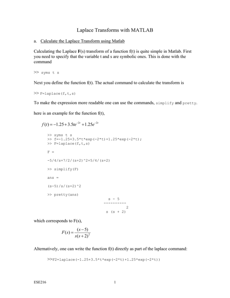
Laplace Transforms with MATLAB
a. Calculate the Laplace Transform using Matlab
Calculating the Laplace F(s) transform of a function f(t) is quite simple in Matlab. First
you need to specify that the variable t and s are symbolic ones. This is done with the
command
>> syms t s
Next you define the function f(t). The actual command to calculate the transform is
>> F=laplace(f,t,s)
To make the expression more readable one can use the commands, simplify and pretty.
here is an example for the function f(t),
f (t ) = −1.25 + 3.5te −2t + 1.25e −2t
>> syms t s
>> f=-1.25+3.5*t*exp(-2*t)+1.25*exp(-2*t);
>> F=laplace(f,t,s)
F =
-5/4/s+7/2/(s+2)^2+5/4/(s+2)
>> simplify(F)
ans =
(s-5)/s/(s+2)^2
>> pretty(ans)
s - 5
---------2
s (s + 2)
which corresponds to F(s),
F ( s) =
( s − 5)
s ( s + 2) 2
Alternatively, one can write the function f(t) directly as part of the laplace command:
>>F2=laplace(-1.25+3.5*t*exp(-2*t)+1.25*exp(-2*t))
ESE216
1
b. Inverse Laplace Transform
The command one uses now is ilaplace. One also needs to define the symbols t and s.
Lets calculate the inverse of the previous function F(s),
F ( s) =
( s − 5)
s ( s + 2) 2
>> syms t s
>> F=(s-5)/(s*(s+2)^2);
>> ilaplace(F)
ans =
-5/4+(7/2*t+5/4)*exp(-2*t)
>> simplify(ans)
ans =
-5/4+7/2*t*exp(-2*t)+5/4*exp(-2*t)
>> pretty(ans)
- 5/4 + 7/2 t exp(-2 t) + 5/4 exp(-2 t)
Which corresponds to f(t)
f (t ) = −1.25 + 3.5te −2t + 1.25e −2t
Alternatively one can write
>> ilaplace((s-5)/(s*(s+2)^2))
Here is another example.
F (s) =
10( s + 2)
s ( s 2 + 4s + 5)
>> F=10*(s+2)/(s*(s^2+4*s+5));
>> ilaplace(F)
ans =
-4*exp(-2*t)*cos(t)+2*exp(-2*t)*sin(t)+4
Which gives f(t),
f (t ) = [4 − 4e −2t cos(t ) + 2e −2t sin(t )]u (t )
making use of the trigonometric relationship,
x sin(α ) + y cos(α ) = R sin(α + β )
and
x cos(α ) − y sin(α ) = R cos(α + β )
with
R = x2 + y2
β = tan −1 ( y / x)
One can also write that f(t) = [4 + 4.47e −2t cos(t − 153.4o )]u (t )
ESE216
2
Matlab often gives the inverse Laplace Transform in terms of sinhx and coshx. Using the
following definition one can rewrite the hyperbolic expression as a function of
exponentials:
ex + e−x
sinh( x) =
2
x
e − e−x
cosh(s ) =
2
Also, you may find the “Heaviside(t) function which corresponds to the unit step function
u(t): thus the function H(t) = heaviside(t) =0 for t<0 and H(t) = heaviside(t)=1 for t>0.
As an example, suppose that Matlab gives you the following result for the inverse
Laplace transform:
2 heaviside(t-10) exp(-5/2t+25) sinh(1/2t-5)
This can be re-written, using the definition of the sinh(x) function:
2u(t)
e 0.5t −5 − e −2.5t +5
] = u (t − 10).e −2.5t + 25+0.5t −5 − e −2.5t + 25−0.5t +5
2
−3t + 30
−e
]
f (t ) = 2u (t − 10).e − 2.5( t −10 ) [
= u (t − 10)[e − 2t + 20
= [e − 2 ( t −10 ) − e −3( t −10 ) ]u (t − 10)
This last expression is closer to what your hand calculations will give you for the invers
Laplace Transform.
ESE216
3