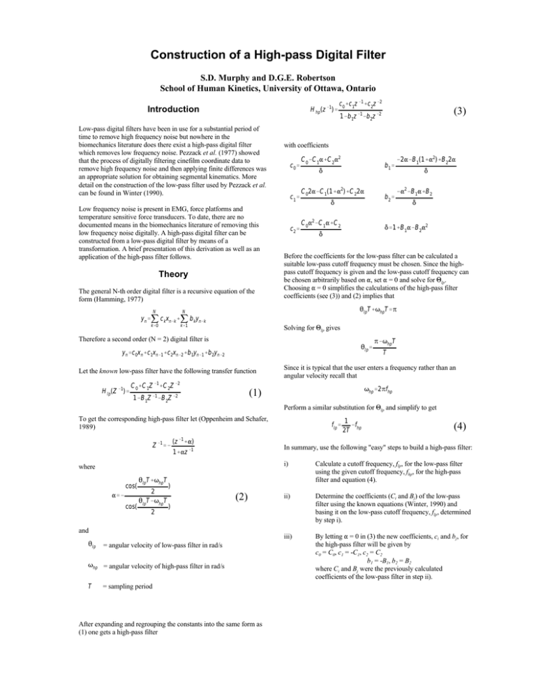
Construction of a High-pass Digital Filter
S.D. Murphy and D.G.E. Robertson
School of Human Kinetics, University of Ottawa, Ontario
H hp(z &1)'
Introduction
Low-pass digital filters have been in use for a substantial period of
time to remove high frequency noise but nowhere in the
biomechanics literature does there exist a high-pass digital filter
which removes low frequency noise. Pezzack et al. (1977) showed
that the process of digitally filtering cinefilm coordinate data to
remove high frequency noise and then applying finite differences was
an appropriate solution for obtaining segmental kinematics. More
detail on the construction of the low-pass filter used by Pezzack et al.
can be found in Winter (1990).
Low frequency noise is present in EMG, force platforms and
temperature sensitive force transducers. To date, there are no
documented means in the biomechanics literature of removing this
low frequency noise digitally. A high-pass digital filter can be
constructed from a low-pass digital filter by means of a
transformation. A brief presentation of this derivation as well as an
application of the high-pass filter follows.
Theory
The general N-th order digital filter is a recursive equation of the
form (Hamming, 1977)
N
k'0
k'1
with coefficients
c0'
c1'
c2'
C0&C1"%C2"2
C02"&C1(1%"2)%C22"
*
C0"2&C1"%C2
2
(z &1%")
1
&f
2T hp
(4)
i)
Calculate a cutoff frequency, flp, for the low-pass filter
using the given cutoff frequency, fhp, for the high-pass
filter and equation (4).
ii)
Determine the coefficients (Ci and Bj) of the low-pass
filter using the known equations (Winter, 1990) and
basing it on the low-pass cutoff frequency, flp, determined
by step i).
iii)
By letting " = 0 in (3) the new coefficients, ci and bj, for
the high-pass filter will be given by
c0 = C0, c1 = -C1, c2 = C2
b1 = -B1, b2 = B2
where Ci and Bj were the previously calculated
coefficients of the low-pass filter in step ii).
)
(2)
)
= angular velocity of low-pass filter in rad/s
Thp = angular velocity of high-pass filter in rad/s
T
flp'
In summary, use the following "easy" steps to build a high-pass filter:
1%"z &1
and
2lp
T
Perform a similar substitution for 1lp and simplify to get
where
cos(
B&ThpT
Thp'2Bfhp
To get the corresponding high-pass filter let (Oppenheim and Schafer,
1989)
2
2lpT&ThpT
*
Since it is typical that the user enters a frequency rather than an
angular velocity recall that
(1)
1&B1Z &1&B2Z &2
"'&
&"2&B1"%B2
Before the coefficients for the low-pass filter can be calculated a
suitable low-pass cutoff frequency must be chosen. Since the highpass cutoff frequency is given and the low-pass cutoff frequency can
be chosen arbitrarily based on ", set " = 0 and solve for 1lp.
Choosing " = 0 simplifies the calculations of the high-pass filter
coefficients (see (3)) and (2) implies that
2lp'
C0%C1Z &1%C2Z &2
2lpT%ThpT
*
Solving for 1lp gives
Let the known low-pass filter have the following transfer function
cos(
b2'
&2"&B1(1%"2)%B22"
*'1%B1"&B2"2
*
y n'c0x n%c1xn&1%c2xn&2%b1yn&1%b2yn&2
Z &1'&
b1'
*
Therefore a second order (N = 2) digital filter is
Hlp(Z &1)'
(3)
1&b1z &1&b2z &2
2lpT%ThpT'B
y n'j c kxn&k%j b kyn&k
N
c0%c1z &1%c2z &2
= sampling period
After expanding and regrouping the constants into the same form as
(1) one gets a high-pass filter
Procedures
The high-pass filter was constructed from a Butterworth, critically
damped, low-pass filter as described by Winter (1990). A typical
EMG signal which had drift present was high-pass filtered in the
forward and backward directions (zero phase lag, 4-th order) with
cutoff frequencies of 0.2 and 0.5 Hz.
Results and Discussion
In Figure 1, the raw EMG signal is plotted above the high-pass
filtered signals with cutoff frequencies of 0.2 and 0.5 Hz. Notice that
a cutoff frequency of 0.2 Hz (middle curve) removed the drift from
the EMG signal. The cutoff of 0.5 Hz removed both the drift and the
bias from the signal without adversely influencing the high frequency
components of the signal. These results demonstrate the usefulness of
a high-pass filter for removing unwanted low frequency noise from
EMG signals.
Figure 2 shows the results of both high and low pass filtering a signal
containing 0.1, 1.0 and 10.0 Hz sine waves. The top curve is the raw
data, the next curve shows the data high-pass filtered at 0.5 Hz cutoff,
the third curve shows the effects of low-pass filtering at 5.0 Hz. The
Figure 1
Figure 2
bottom curve shows the effects of cascading the data through a 0.5
Hz high-pass filter and a 5.0 Hz low-pass filter. This band-pass filter
successfully recovered the 1.0 Hz sine wave from the raw signal.
Notice that these filters do require time to reach their specified
operating characteristics. In this case (zero phase lag filters) extra
leading and trailing data are required (see Smith, 1989).
References
Hamming, R.W. (1977) Digital filters. Prentice-Hall, Inc.
Oppenheim, A.V. and Schafer, R.W. (1989) Discrete-time signal
processing.
Pezzack, J.C. et al. (1977) J. Biomechanics, 10, 377-382.
Smith, G. (1989) J. Biomechanics, 22, 967-972.
Winter, D.A. (1990) Biomechanics and motor control of human
movement. John Wiley & Sons.
Acknowledgments
For technical assistance, thanks to Dr. Tyseer Aboulnasr, Dept.
Electrical Engineering, U.Ottawa. For use of data, thanks to Dr.
Mario Lamontagne, School of Human Kinetics, U. Ottawa.