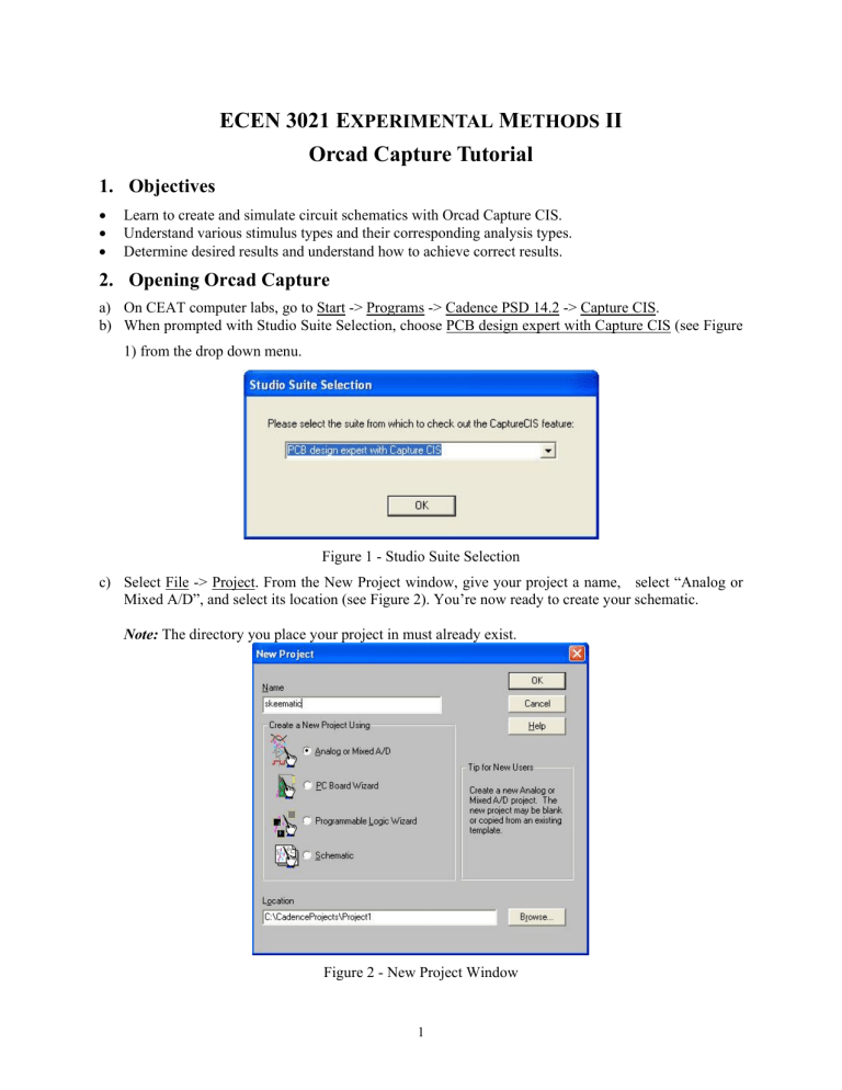
Orcad Capture Tutorial

ECEN 3021 E
XPERIMENTAL
M
ETHODS
II
Orcad Capture Tutorial
1.
Objectives
•
•
Learn to create and simulate circuit schematics with Orcad Capture CIS.
Understand various stimulus types and their corresponding analysis types.
•
Determine desired results and understand how to achieve correct results.
2.
Opening Orcad Capture
a) On CEAT computer labs, go to Start -> Programs -> Cadence PSD 14.2 -> Capture CIS. b) When prompted with Studio Suite Selection, choose PCB design expert with Capture CIS (see Figure
1) from the drop down menu.
Figure 1 - Studio Suite Selection c) Select File -> Project. From the New Project window, give your project a name, select “Analog or
Mixed A/D”, and select its location (see Figure 2). You’re now ready to create your schematic.
Note: The directory you place your project in must already exist.
Figure 2 - New Project Window
1
3.
Creating Schematics with Capture CIS
a) Next we must draw the desired schematic. To get parts, go to Place -> Part…(see Figure 3). Shift+P allows us to reach this dialog box quickly.
Note: If no parts are visible in the “Place Part” dialog, simply click on the “Add Library…” button.
Inside the Browse File dialog, click on any *.olb file the press Ctrl+A to select all the files (or
Ctrl+Arrow to select certain library files) and hit the “Open File” button.
Note: The library files we will be using should be in the directory
C:\Cadence\PSD_14.2\tools\capture\library\pspice
Figure 3 - Place Part Dialog b) Let’s draw a simple RLC circuit. We will find the parts we need by typing the name of the part in the
Part section and clicking “OK.” So, let’s draw the circuit below.
R2
100
V1 = 0
V2 = 10
TD = 1u
TR = 1p
TF = 1p
PW = 1u
PER =
V1
R1
10k
C1
0.01u
L1
150mH
0
2
c) Remember we always need a ground in the circuit, this can be found in the Place Ground menu, accessible by clicking the button on the right side of the screen. The ground we will use is the
0/SOURCE identified by the symbol . d) Moving, rotating, and other part manipulation functions can be accomplished through the Edit menu at the top of the screen or right click with part selected.
Warning: When making changes be careful, else parts may become disconnected.
4.
Circuit Simulation
a) After all desired components are in place, go to PSpice -> New Simulation Profile. (see Figure 4).
Name your simulation profile and click on Create, then the “Simulation Settings” (see Figure 5) dialog will appear.
Figure 4 - Naming Simulation
Figure 5 - Simulation Settings
3
b) Select the correct analysis type for desired output. Then further change the options for a more specific analysis. Once desired options are selected, click “OK.” To actually run the simulation, select PSpice
-> Run.
5.
Types of Stimulus and Analysis
Each type of source is actually paired with a certain type of analysis, and in most cases with only one. The primary sources we will use in this class are VPulse, Vsin, and Vac. These are available in the standard
PSpice libraries you added when you created the schematic.
5.1
VPulse
It is used to measure the transient response of a circuit. For Vpulse, we control all aspects of generated pseudo-square wave. Factors directly affecting produced Vpulse function are visible in Table 1 below.
Table 1 Vpulse characteristics [1]
Pulse Parameter
V1
V2
TD
TR
TF
Explanation
Starting voltage for pulse
Second voltage for pulse
Time delay. Voltage will remain at V1 until this specified time.
Rise time. Time required to reach V2 from V1 (Rise time must not equal zero).
Fall time. Time required for voltage to change from V2 to V1 (Again, fall time must not be equal to zero).
Pulse width. Amount of time pulse remains at V2.
Period of pulse. How often pulse actually repeats itself
PW
PER a) VPulse combined with the Time domain (transient) analysis. Let’s take the following example of an
RLC network. First draw the following circuit.
R2
100
V1 = 0
V2 = 10
TD = 1u
TR = 1p
TF = 1p
PW = 1u
PER =
V1
R1
10k
C1
0.01u
L1
150mH
0
Now it is time to change the Simulation Settings to the desired values. We can access the settings by clicking on the button. So, we will find that value and in turn set the Run to time to approximately 10 us. As can be see from the Time Domain simulation below, the output is trying to follow the input and at the end, the output reaches the steady state value of 0 Volts after input becomes zero.
4
5.2
Vsin
This source, used in conjunction with the transient sweep, yields the time response of a circuit with a constant frequency input. Vsin has the parameters: Voff (Offset Voltage), Vampl (Amplitude), and Freq
(Frequency). In what circumstances could this tool be useful to us? What kind of response should we expect? a) Let’s take the following example. Once drawn, we’ll again use the Time Domain (transient) sweep as we did in the section above. Select a running time of approximately 100 ms, just so we can see beyond the point where the sine wave crosses 0 volts.
IN R2 OUT
10k
V2
VOFF = 0
VAMPL = 5
FREQ = 60
C1
0.5u
0 b) But wait a second, what are those funny little bubble things? They are a trick to naming the wires that they are attached to. They’re guaranteed to make our life easier. Simply find the button on the right of the screen. Once in the Place Power menu find VCC/CAPSYM identified by let’s just change their names.
. Now, c) Since we already have the desired simulation settings, let’s simulate by clicking the button, or by pressing F11. PSpice A/D will appear as before but nothing will be present. So we will need to find the appropriate waveforms to add.
5
d) Click on the button. Once the Add Trace dialog is open, find V(IN) and V(OUT). Multiple traces can be added (when separated by commas, as visible in Figure 6.
Figure 6 - Add Trace Dialog
Our output is now visible as seen in Figure 7, below. Are the results as we expected? How can we be sure we conducted the correct analysis? Finally, what does the following graph mean?
Figure 7 - Vsin Transient Sweep
To have the smooth curves, change the default maximum step size equal to 10u seconds in the Simulation
Settings. Observe the curve, is it smooth or not? If not then reduce the step size more. If simulations are taking a very long time, then increase the step size.
6
6.
Output Display options
We now know how to get the desired results based on either a circuit’s response to either change in time or frequency. Let’s take what we’ve learned and find some ways to transform our output data to allow us to gather exactly the information we need from our circuit.
6.1
Gain/Attenuation
Gain or attenuation is a measure of how much of a signal actually passes through a circuit. In many amplifiers which you have already constructed, you have witnessed gain. Gain is defined by V out
/V in
.
Let’s see if we can find the gain for a simple RLC circuit. a) Let’s draw the circuit below and find the smooth output.
IN R2 OUT
1k
V2
VOFF = 0
VAMPL = 5
FREQ = 60
R3
1k
0 b) Remember that we want to use the Time Domain analysis with our Vac source; otherwise we might not get any results. Are these the results we expected? c) What of the relationship between the output and input? Let’s use the above definition of gain and find the exact gain for this circuit. First, we’ll keep both of these traces and go back to the Add Trace button. In the Trace Expression window, we’ll divide one waveform by the other as shown . Next we just have to click “OK.” Did we expect the graph below? What kind of information does this give us?
7
d) Another useful way to illustrate gain or attenuation is with the use of decibels. Decibels are best defined as the level of relative strength of a signal. Follow the directions, but from the Functions or
Macros section of the Add Trace window select Analog Operators and Functions in the drop down menu. Now select DB() from the list, and make sure the following appears in the Trace Expression window: then just click on "OK." What did you observe?
7.
Exercises
We now have the basic analysis tools for the circuits. We will be using PSpice extensively in this class.
Go ahead and analyze the circuits in the lab exercise.
8
