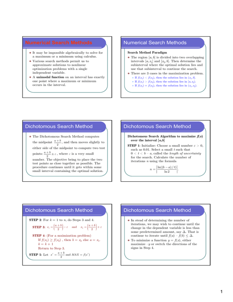
Numerical Search Methods
z
z
z
It may be impossible algebraically to solve for
a maximum or a minimum using calculus.
Various search methods permit us to
approximate solutions to nonlinear
optimization problems with a single
independent variable.
A unimodal function on an interval has exactly
one point where a maximum or minimum
occurs in the interval.
Dichotomous Search Method
z
The Dichotomous Search Method computes
a +b
the midpoint
, and then moves slightly to
2
either side of the midpoint to compute two test
points: a + b ± ε , where ε is a very small
2
number. The objective being to place the two
test points as close together as possible. The
procedure continues until it gets within some
small interval containing the optimal solution.
Dichotomous Search Method
STEP 2: For k = 1 to n, do Steps 3 and 4.
⎛a + b ⎞⎟
STEP 3: x 1 = ⎜⎜⎝
⎟− ε
2 ⎠⎟
and
Search Method Paradigm
z The region [a, b] is divided into two overlapping
intervals [a, x1] and [x2, b]. Then determine the
subinterval where the optimal solution lies and
use that subinterval to continue the search.
z There are 3 cases in the maximization problem.
z
z
z
If f (x1) < f (x2), then the solution lies in (x1, b].
If f (x1) > f (x2), then the solution lies in [a, x2).
If f (x1) = f (x2), then the solution lies in (x1, x2).
Dichotomous Search Method
Dichotomous Search Algorithm to maximize f(x)
over the interval [a,b]
STEP 1: Initialize: Choose a small number ε > 0,
such as 0.01. Select a small t such that
0 < t < b – a, called the length of uncertainty
for the search. Calculate the number of
iterations n using the formula
⎡ ln((b − a )/ t ) ⎤
⎥.
n=⎢
ln 2
⎢⎢
⎥⎥
Dichotomous Search Method
z
⎛a + b ⎞⎟
x 2 = ⎜⎜
+ε
⎝ 2 ⎠⎟⎟
STEP 4: (For a mximization problem)
If f (x1) ≥ f (x2) , then b = x2 else a = x1.
k=k+1
Return to Step 3.
STEP 5: Let x * =
Numerical Search Methods
z
In stead of determining the number of
iterations, we may wish to continue until the
change in the dependent variable is less than
some predetermined amount, say Δ. That is
continue to iterate until f (a) – f (b) ≤ Δ.
To minimize a function y = f (x), either
maximize –y or switch the directions of the
signs in Step 4.
a +b
and MAX = f (x * )
2
1
Dichotomous Search Method
Example
Maximize f (x) = –x2 – 2x over the interval
–3 ≤ x ≤ 6. Assume the optimal tolerance to
be less than 0.2 and we choose ε = 0.01.
z We determine the number of iterations to be
⎡ ⎛ 6 − (−3)⎞ ⎤
⎟⎟ ⎥
⎢ ln ⎜⎜
⎢ ⎝⎜ 0.2 ⎠⎟ ⎥ ⎡ ln 45 ⎤
⎥=⎢
n=⎢
⎥ = ⎡5.49⎤ = 6
ln 2
⎢
⎥ ⎢ ln 2 ⎥
Golden Section Search Method
z
z
The Golden Section Search Method chooses x1
and x2 such that the one of the two evaluations
of the function in each step can be reused in
the next step.
The golden ratio is the ratio r satisfying
r
1−r
=
1
r
⇒
r=
5 −1
≈ 0.618034
2
r
(1 − r )
Golden Section Search Method
Golden Section Search Method to maximize
f (x) over the interval a ≤ x ≤ b.
STEP 1: Initialize: Choose a tolerance t > 0.
5 −1
STEP 2: Set r =
and define the test
2
points:
x 1 = a + (1 − r ) (b − a )
x 2 = a + r (b − a )
STEP 3: Calculate f (x1) and f (x2).
Dichotomous Search Method
Results of a Dichotomous Search.
z
n
a
b
x1
x2
f (x1)
f (x2)
0
–3
6
1.49
1.51
– 5.2001
– 5.3001
1
–3
1.51
– 0.755
– 0.735
0.939975
0.929775
2
–3
– 0.735
– 1.8775
– 1.8575
0.229994
0.264694
3
– 1.8775
– 0.735
– 1.31625
– 1.29625
0.899986
0.912236
4
– 1.31625
– 0.735
– 1.03563
– 1.01563
0.998731
0.999756
5
– 1 .03563
– 0.735
– 0.89531
– 0.87531
0.989041
0.984453
6
– 1.03563
– 0.87531
x* =
−1.03563 − 0.87531
= −0.95547 and f (x * ) = 0.99802
2
Golden Section Search Method
y
r1 =
b − x1
r2 =
b −a
x1
a
r1 =
x2
b
1 − r2
r1
and
r2 =
r1 = r2 =
5 −1
2
1 − r1
r2
x
x2 − a
b −a
Golden Section Search Method
STEP 4: (For a maximization problem)
If f (x1) ≤ f (x2) then a = x1, x1 = x2
else b = x2, x2 = x1. Find the new x1 or x2
using the formula in Step 2.
STEP 5: If the length of the new interval from
Step 4 is less than the tolerance t specified,
then stop. Otherwise go back to Step 3.
STEP 6: Estimate x* as the midpoint of the final
interval x * =
a +b
and compute MAX = f (x*)
2
2
Golden Section Search Method
z
z
z
To minimize a function y = f (x), either
maximize –y or switch the directions of the
signs in Step 4.
The advantage of the Golden Section Search
Method is that only one new test point must
be computed at each successive iteration.
The length of the uncertainty is 61.8% of he
length of the previous interval of uncertainty.
Golden Section Search Method
n
a
b
x1
x2
f (x1)
f (x2)
0
-3
6
0.437694
2.562306
-1.06696
-11.69
1
-3
2.562306
-0.87539
0.437694
0.984472
-1.06696
2
-3
0.437694
-1.68692
-0.87539
0.528144
0.984472
3
-1.68692
0.437694
-0.87539
-0.37384
0.984472
0.607918
4
-1.68692
-0.37384
-1.18536
-0.87539
0.96564
0.984472
5
-1.18536
-0.37384
-0.87539
-0.68381
0.984472
0.900025
6
-1.18536
-0.68381
-0.99379
-0.87539
0.999961
0.984472
7
-1.18536
-0.87539
-1.06696
-0.99379
0.995516
0.999961
8
-1.06696
-0.87539
-0.99379
-0.94856
0.999961
0.997354
9
-1.06696
-0.94856
-1.02174
-0.99379
0.999527
0.999961
10
-1.02174
-0.94856
-0.99379
-0.97651
0.999961
0.999448
11
-1.02174
-0.97651
x * = −0.99913
Golden Section Search Method
How small should the tolerance be?
If x * is the optimal point, then
f (x ) ≈ f (x * ) +
If we want the second term to be of a fraction
ε of the first term, then
2 f (x * )
(x * )2 f ′′(x * )
MAX = 0.999999
Fibonacci Search Method
z If
1
f ′′(x * )(x − x * )2 .
2
x − x* = ε x*
and
a number of test points is specified in
advanced, then we can do slightly better
than the Golden Section Search Method.
z This method has the largest interval
reduction compared to other methods
using the same number of test points.
.
As a rule of thumb, we need x − x * ≈ ε x * .
Fibonacci Search Method
Fibonacci Search Method
I n −2
I n −1
In
αI n = εI 1
αI n
xn
In =
x n −1
x n −2
1
1
I n −1 + αI n
2
2
⇒
f (x n −2 ) > f (x n −3 )
In
In
xn
I n −1 = (2 − α)I n
f (x n −1 ) > f (x n −2 )
I n −1
f (x n −1 ) > f (x n −2 )
In
x n −1
x n −2
x n −3
I n −2 = I n −1 + I n = (2 − α)I n + I n = (3 − α)I n
3
Fibonacci Search Method
Fibonacci Search Method
I n −1 = (2 − α)I n
I 1 = (Fn +1 − Fn −1α)I n = Fn +1I n − Fn −1 (εI 1 )
I n −2 = I n −1 + I n = (2 − α)I n + I n = (3 − α)I n
I1
I n −3 = I n −2 + I n −1 = (3 − α)I n + (2 − α)I n = (5 − 2α)I n
I n −4 = I n −3 + I n −2 = (5 − 2α)I n + (3 − α)I n = (8 − 3α)I n
I3
I2
#
x1
a
I n −k = (Fk +2 − Fk α)I n
⎛1 + F ε ⎞⎟
n −1
⎟I
I n = ⎜⎜⎜
⎜⎝ Fn +1 ⎠⎟⎟ 1
I2
I3
x2
b
x 1 = a + I 3 = a + (Fn −1 + Fn −3 α ) I n = a + Fn −1I n + Fn −3 (εI 1 )
where Fk +2 = Fk +1 + Fk , F1 = F2 = 1
Fibonacci Search Method
z If
ε = 0, then the formula simplify to
In =
I1
Fn +1
Fn −1
(b − a )
Fn +1
F
x 2 = a + n (b − a )
Fn +1
x1 = a +
x 2 = a + I 2 = a + (Fn + Fn −2 α ) I n = a + Fn I n + Fn −2 (εI 1 )
Fibonacci Search Method
Fibonacci Search Method to maximize
f (x) over the interval a ≤ x ≤ b.
STEP 1: Initialize: Choose the number of test
points n.
STEP 2: Define the test points:
x1 = a +
Fn −1
F
(b − a ), x 2 = a + n (b − a )
Fn +1
Fn +1
STEP 3: Calculate f (x1) and f (x2).
Fibonacci Search Method
STEP 4: (For a maximization problem)
If f (x1) ≤ f (x2) then a = x1, x1 = x2
else b = x2, x2 = x1.
n = n – 1. Find the new x1 or x2 using the
formula in Step 2.
STEP 5: If n > 1, return to Step 3.
STEP 6: Estimate x* as the midpoint of the final
a +b
interval x * =
2
and compute MAX = f (x*)
Fibonacci Search Method
n
Fn
13
233
a
b
x1
x2
f (x1)
f (x2)
-11.6895
12
144
-3
6
0.437768
2.562232
-1.06718
11
89
-3
2.562232
-0.87554
0.437768
0.984509
10
55
-3
0.437768
-1.6867
-0.87554
0.52845
0.984509
9
34
-1.6867
0.437768
-0.87554
-0.37339
0.984509
0.607361
8
21
-1.6867
-0.37339
-1.18455
-0.87554
0.965942
0.984509
7
13
-1.18455
-0.37339
-0.87554
-0.6824
0.984509
0.899132
6
8
-1.18455
-0.6824
-0.99142
-0.87554
0.999926
0.984509
5
5
-1.18455
-0.87554
-1.06867
-0.99142
0.995284
0.999926
4
3
-1.06867
-0.87554
-0.99142
-0.95279
0.999926
0.997771
3
2
-1.06867
-0.95279
-1.03004
-0.99142
0.999097
0.999926
2
1
-1.03004
-0.95279
-0.99142
-0.99142
0.999926
0.999926
1
1
-1.03004
-0.99142
x * = −1.01073
and
-1.06718
MAX = 0.999885
4