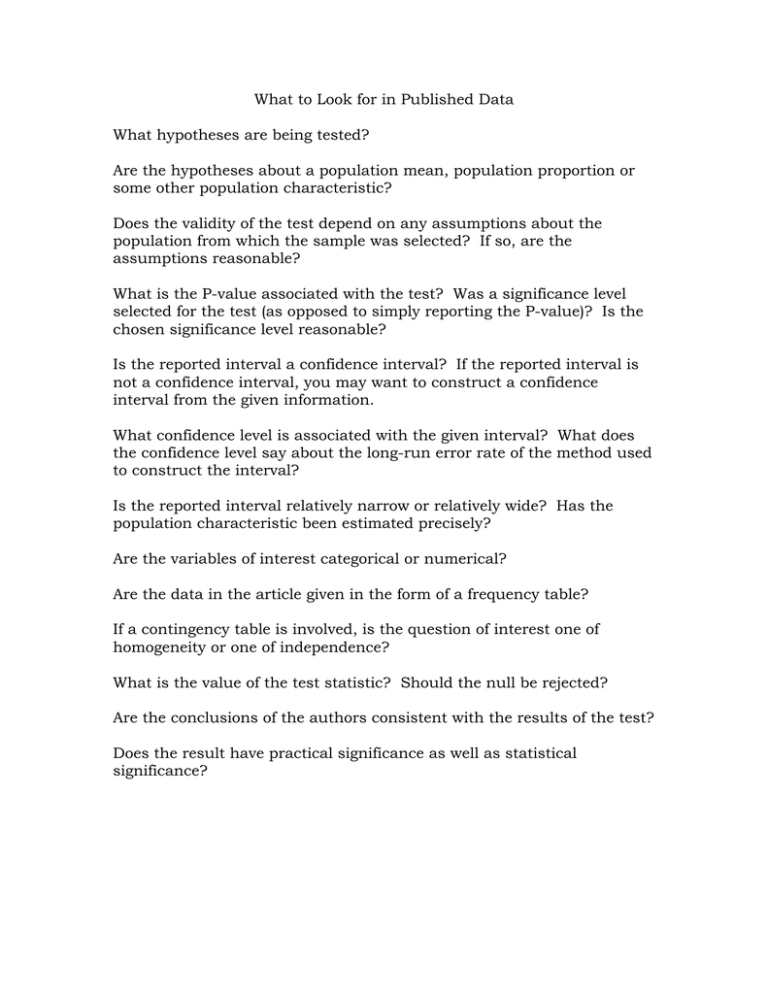
What to Look for in Published Data
What hypotheses are being tested?
Are the hypotheses about a population mean, population proportion or
some other population characteristic?
Does the validity of the test depend on any assumptions about the
population from which the sample was selected? If so, are the
assumptions reasonable?
What is the P-value associated with the test? Was a significance level
selected for the test (as opposed to simply reporting the P-value)? Is the
chosen significance level reasonable?
Is the reported interval a confidence interval? If the reported interval is
not a confidence interval, you may want to construct a confidence
interval from the given information.
What confidence level is associated with the given interval? What does
the confidence level say about the long-run error rate of the method used
to construct the interval?
Is the reported interval relatively narrow or relatively wide? Has the
population characteristic been estimated precisely?
Are the variables of interest categorical or numerical?
Are the data in the article given in the form of a frequency table?
If a contingency table is involved, is the question of interest one of
homogeneity or one of independence?
What is the value of the test statistic? Should the null be rejected?
Are the conclusions of the authors consistent with the results of the test?
Does the result have practical significance as well as statistical
significance?
Example 1
Consider the following statement (based on information in the article
“Serum Transferrin Receptor for the Detection of Iron Deficiency in
Pregnancy,” (American Journal of Clinical Nutrition [1991]: 1077 – 1081):
“In a total sample of 176 pregnant women, mean serum receptor
concentration did not differ significantly from 5.63, the mean for women
who are not pregnant (P>0.10).”
The statement does not indicate what test was performed or what the
value of the test statistic was. It appears that the hypotheses of interest
are H 0 :   5.63 versus H a :   5.63 , where  represents the true mean
serum receptor concentration for pregnant women. Because the sample
size is large, the one-sample t test would be appropriate if the sample
can be considered a random sample. With the large sample size, no
assumptions abut the shape of the population distribution of serum
receptor concentration values are necessary. Because the reported Pvalue is so large (P-value>0.10), there is no reason to reject H 0 . We
cannot conclude that the mean for pregnant women differs from the
known mean of 5.63 for women who are not pregnant.
Example 2
Consider the article “Increased Vital and Total Lung Capacity in Tibetan
Compared to Han Residents of Lhasa” (American Journal of Physical
Anthropology [1991]:mm341 – 351) that compared various physical
characteristics of people who lived at high altitudes with those of people
who live at sea level. The article includes the following statements: “We
studied 38 Tibetan and 43 Han residents….The Tibetan compared with
the Han subjects had a larger total lung capacity
6.80  0.19 (mean  SEM) vs. 6.24  0.18 liters .” SEM means standard error of
the mean not margin of error.
The report intervals are of the form estimate  standard error . We can use
this information to construct a confidence interval for the mean total
lung capacity for residents of each of the two locations. Because the
sample sizes are both large, we can use the t confidence interval formula
mean   t critical value standard deviation of the mean 
The Tibetan sample has df = 38 – 1 =37 and
The Han sample has df = 43 – 1 = 42.
The 95% confidence intervals are
Tibetan residents: 6.80  2.03  0.19   6.41,7.19
Han residents: 6.24  2.02  0.18   5.88,6.60
Assuming that it is reasonable to view these samples as random
samples, we can interpret these intervals as follows: Based on the
information provided in the sample of Tibetan residents, we can be 95%
confident that the mean total lung capacity of Tibetan residents is
between 6.42 and 7.18, and based on the information provided in the
sample of Han residents, we can be 95% confident that the mean total
lung capacity of Han residents is between 5.88 and 6.60. These intervals
are not very narrow, indicating that the value of the population mean has
not been estimated as precisely as we might like in either case. This is
not surprising, given the reported sample sizes and the variability in each
sample. Not that the two intervals overlap. This may cause us to be
skeptical of the statement that Tibetans have a higher total lung capacity
than Han residents. Formal methods for directly comparing two groups
(2-sample t interval) should used to further investigate this issue.
Example 3
Consider a study reported in the article “The Relationship Between
Distress and Delight in Males’ and Females’ Reaction to Frightening
Films” (Human Communication Research [1991]: 625 – 637). The
investigation measured emotional responses of 50 males and 60 females
after the subjects viewed a segment from a horror film. The article
included the following statement: “Females were much more likely to
express distress than were males. While males did express higher levels
of delight than females, the difference was not statistically significant.”
The following summary information was also contained in the article:
GENDER
Males
Females
DISTRESS INDEX
Mean
SD
31.2
10.0
40.4
9.1
P-value<.001
DELIGHT INDEX
Mean
SD
12.02
3.65
9.09
5.55
Not significant
P-value>.05
The P-values are the only evidence of the hypothesis tests that support
the given conclusions. The P-value<.001 for the distress index means
that the hypothesis H 0 : F  M  0 was rejected in favor of H 0 : F  M  0 .
The nonsignificant P-value (P-value>.05) reported for the delight index
means that the hypothesis H 0 : F  M  0 could not be rejected. Chance
sample-to-sample variability is a plausible explanation for the observed
difference in sample means (12.02 – 9.09). Thus we would not want to
put much emphasis on the author’s statement that males express higher
levels of delight than females, because it is based only on the fact that
12.02>9.09, which could plausibly be due entirely to chance.
The article describes the samples as consisting of undergraduates
selected from the student body of a large Midwestern university. The
authors extrapolate their results to American men and women in general.
If this type of generalization is considered unreasonable, we could be
more conservative and view the sampled populations as male and female
university students or even male and female students at this university.
The comparison of males and females was based on two independently
selected groups (not paired). Because the sample sizes were large, the 2sample t test for means could reasonably have been used, and this would
have required no specific assumptions abut the two underlying
populations.
Example 4
The authors of the article “Predicting Professional Sports Game Outcomes from
Intermediate Game Scores” (Chance [1992]: 18-22) used a chi-square test to determine
whether there was any merit to the idea that basketball games were not settled until the
last quarter, whereas baseball games are over the seventh inning. They also
considered football and hockey. Data were collected for 189 basketball games, 92
baseball games, 80 hockey games, and 93 football games. The analyzed games were
sampled randomly from all games played during the 1990 season for baseball and
football and for the 1990 – 1991 season for basketball and hockey. For each game, the
late-game leader was determined, and then it was noted whether the late-game leader
actually ended up winning the game. The resulting data are summarized in the
following table.
Sport
Basketball
Baseball
Hockey
Football
Late-Game
Leader
2Wins
150
86
65
72
Late-Game
Leader
Loses
39
6
15
21
The authors stated that the “late-game leader us defined as the team that is ahead after
three quarters in basketball and football, two periods in hockey, and seven innings in
baseball. The chi-square value (with three degrees of freedom) is 10.52 (P<.015).” They
also concluded that “the sport that is an anomaly is baseball. Only 6.5% of baseball
games resulted in late reversals…. [The chi-square test] is statistically significant due
almost entirely to baseball.
In this particular analysis, the authors are comparing four populations (games from
each of the four sports) on the basis of a categorical variable with tow categories (lategame leader wins and late-game leader loses). The appropriate null hypothesis is then
H 0 : The true proportion in each category (leader wins, leader loses) is the same for all four sports.
Based on the reported value of the chi-square statistic and the associated P-value, this
null hypothesis is rejected, leading to the conclusion that the category proportions are
not the same for all four sports.
The validity of the chi-square test requires that the sample sizes be large enough so that
no expected counts are less than 5. The smallest expected count is 14.27, so the
sample sizes are large enough to justify the use of the
2
X 2 test. Note also that baseball
contributes a total of 8.042 to the value of the X statistic of 10.518. This is due to the
large discrepancies between the observed and expected counts in the other cells. This
is probably the basis for the authors’ conclusion that baseball is the only anomaly and
that the other sports were similar.
AP Statistics Project (1)
Due: 4/23/10
Part 1
Find and attach full copies of two related journal articles that use
statistical inference to support their position or findings. The articles do
not have to come from the same publication. The articles should be on
the same or similar topic. Please have me approve your articles before
you proceed to step 2 and 3.
Part 2
Look for the statistical features in one of the articles. Attached is a list
(set of questions) of some of the features. Also attached are four
examples of how to analyze the articles.
Part 3
Report on one of the two articles:
Your report is oral and in the form of a Power Point presentation. Prepare
your Power Point presentation as per the directions below. Place the
presentation into my “STATS” folder on the student common drive by
3:00 pm on 4/23/10.
Power Point presentation should contain:
1. 2 – 3 slides - No more than 10 minute explanation.
2. A brief explanation about the nature and purpose of the research. Be
sure to include the author, title and source.
3. A comment about how the author generalizes to a larger population
based on his sample. Give details about the sample (W’s).
4. An explanation about one of the hypothesis tests performed and the
conclusions drawn. Do you agree? Why?
5. And be ready to answer general questions about the second article.
Name:
1. 2 journal articles appropriate
2. powerpoint and articles submitted on time
3. Power Point presentation should contain:
A. 2 – 3 slides - No more than 10 minute explanation.
B. A brief explanation about the nature and purpose of the research. Be
sure to include the author, title and source.
C. A comment about how the author generalizes to a larger population
based on his sample. Give details about the sample (W’s).
D. An explanation about one of the hypothesis tests performed and the
conclusions drawn. Do you agree? Why?
E. And be ready to answer general questions about the second article.