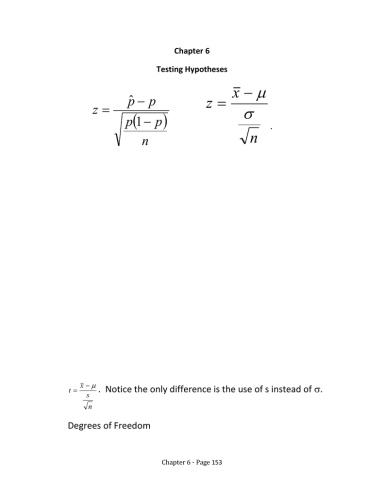
Chapter 6
Testing Hypotheses
z
t
x
s
pˆ  p
p1  p 
n
z
x

n
.
. Notice the only difference is the use of s instead of .
n
Degrees of Freedom
Chapter 6 - Page 153
Student t distributions
One Tail
Probability
0.4
0.25
0.1
0.05
0.025
0.01
0.005
0.0005
Two Tail
Probability
0.8
0.5
0.2
0.1
0.05
0.02
0.01
0.001
Confidence
Level
20%
50%
80%
90%
95%
98%
99%
99.9%
0.325
0.289
0.277
0.271
0.267
0.265
0.263
0.262
0.261
0.260
0.260
0.259
0.259
0.258
0.258
0.258
0.257
0.257
0.257
0.257
0.257
0.256
0.256
0.256
0.256
0.256
0.256
0.256
0.256
0.256
0.255
0.254
0.254
0.253
1.000
0.816
0.765
0.741
0.727
0.718
0.711
0.706
0.703
0.700
0.697
0.695
0.694
0.692
0.691
0.690
0.689
0.688
0.688
0.687
0.686
0.686
0.685
0.685
0.684
0.684
0.684
0.683
0.683
0.683
0.681
0.679
0.677
0.674
3.078
1.886
1.638
1.533
1.476
1.440
1.415
1.397
1.383
1.372
1.363
1.356
1.350
1.345
1.341
1.337
1.333
1.330
1.328
1.325
1.323
1.321
1.319
1.318
1.316
1.315
1.314
1.313
1.311
1.310
1.303
1.296
1.289
1.282
6.314
2.920
2.353
2.132
2.015
1.943
1.895
1.860
1.833
1.812
1.796
1.782
1.771
1.761
1.753
1.746
1.740
1.734
1.729
1.725
1.721
1.717
1.714
1.711
1.708
1.706
1.703
1.701
1.699
1.697
1.684
1.671
1.658
1.645
12.706
4.303
3.182
2.776
2.571
2.447
2.365
2.306
2.262
2.228
2.201
2.179
2.160
2.145
2.131
2.120
2.110
2.101
2.093
2.086
2.080
2.074
2.069
2.064
2.060
2.056
2.052
2.048
2.045
2.042
2.021
2.000
1.980
1.960
31.821
6.965
4.541
3.747
3.365
3.143
2.998
2.896
2.821
2.764
2.718
2.681
2.650
2.624
2.602
2.583
2.567
2.552
2.539
2.528
2.518
2.508
2.500
2.492
2.485
2.479
2.473
2.467
2.462
2.457
2.423
2.390
2.358
2.326
63.656
9.925
5.841
4.604
4.032
3.707
3.499
3.355
3.250
3.169
3.106
3.055
3.012
2.977
2.947
2.921
2.898
2.878
2.861
2.845
2.831
2.819
2.807
2.797
2.787
2.779
2.771
2.763
2.756
2.750
2.704
2.660
2.617
2.576
636.578
31.600
12.924
8.610
6.869
5.959
5.408
5.041
4.781
4.587
4.437
4.318
4.221
4.140
4.073
4.015
3.965
3.922
3.883
3.850
3.819
3.792
3.768
3.745
3.725
3.707
3.689
3.674
3.660
3.646
3.551
3.460
3.373
3.290
df
1
2
3
4
5
6
7
8
9
10
11
12
13
14
15
16
17
18
19
20
21
22
23
24
25
26
27
28
29
30
40
60
120
z*
Chapter 6 - Page 154
Use the table to find a p-value. You will use inequality signs to show
the p-value with as much precision as possible, compared with alpha.
1. H1: >
 = 0.05 df = 12, t = 1.9
2. H1: ≠
 = 0.01 df = 25, t = -1.1
The four hypothesis-test formulas that will be shown in this chapter
will be illustrated with these five questions. As you read the questions,
try to determine any similarities or differences between them, as that
will ultimately guide you into which formula should be used.
 Are more than 10% of households prepared for a natural disaster?
 Is there a difference between the proportion of households in
tornado/hurricane areas prepared for a disaster and the
proportion of households in earthquake areas?
 Is the average daily caloric intake of US residents greater than
3000 kcal?
 Is the average daily caloric intake of Canadian residents less than
the average daily caloric intake of Americans?
 Is there a significant difference between the average daily caloric
intake of a person on a diet compared to prior to the diet?
Chapter 6 - Page 155
Question
Parameter
Populati Hypotheses
ons
Are more than 10% of
households prepared for a
natural disaster?
Is there a difference between
the proportion of households
in tornado/hurricane areas
prepared for a disaster and
the proportion of households
in earthquake areas?
proportion
1
H0: P = 0.1
H1: P > 0.1
proportion
2
H0: PT = PE
H1: PT ≠PE
1
H0: µ = 3000
H1: µ > 3000
1
H0 : µ = 0
H1 : µ ≠ 0
2
H0: µ Canadian = µ
Is the average daily caloric
mean
intake of US residents greater
than 3000 kcal?
Is there a significant
mean
difference between the
average daily caloric intake of
a person on a diet compared
to prior to the diet?
Is the average daily caloric
mean
intake of Canadian residents
less than the average daily
caloric intake of Americans?
.
Chapter 6 - Page 156
American
H1: µ Canadian < µ
American
For Categorical Data Normal Approximation to Binomial
X
XXX
XXXXX
µ =np.
  npq
.
z
x

.
p̂
p̂ p̂ p̂
p̂ p̂ p̂ p̂ p̂
 pˆ  p
 pˆ 
p1  p 
.
n
z
pˆ  p
p1  p 
n
.
Chapter 6 - Page 157
x
x x x
x x x x x
x  
x 

n
.
z
x

. Because  is not known, it is estimated
n
with s, so that the estimated standard error is
is replaced by the t formula where
t
x
s
sx 
s
n
and the Z formula
.
n
Assumptions for the remaining formulas that will not be proved
1. The mean of the difference of two random variables is the difference
of the means.
2. The variance of the difference of two independent random variables
is the sum of the variances.
3. The difference of two independent normally distributed random
variables is also normally distributed.1
1
Aliaga, Martha, and Brenda Gunderson. Interactive Statistics. Upper Saddle River, NJ: Pearson Prentice Hall, 2006.
Print.
Chapter 6 - Page 158
Is there a difference between the proportion of households in
tornado/hurricane areas prepared for a disaster and the proportion of
households in earthquake areas? This means that there are two
populations, the population in tornado/hurricane country and
earthquake country. Within each population, the proportion of people
who are prepared will be found. The hypotheses are:
H0: PT = PE
H1: PT ≠PE
H0 : P T – P E = 0
H1: PTe – PE ≠ 0
Since neither PT or PE is known because these are parameters, the
best that can be done is estimate them using sample proportions.
Therefore p̂T will be used as an estimate of PT and p̂E will be used as an
estimate of PE. Then pˆ T  pˆ E as an estimate for PT – PE.
The distribution of interest to us is the one consisting of the
difference between sample proportions, generically shown as pˆ A  pˆ B .
pˆ A  pˆ B
pˆ A  pˆ B
pˆ A  pˆ B pˆ A  pˆ B
Chapter 6 - Page 159
The mean of this distribution is pA – pB and the standard
deviation is p A 1  p A  p B 1  p B  . Since the only thing that is known
nA

nB
about pA and pB is that they are equal, it is necessary to estimate
their value so that the standard deviation can actually be computed. To
do this, the sample proportions will be combined. The combined
proportion is defined as
pˆ c 
Replacing pA and pB with
standard error of
p̂ c
x A  xB
n A  nB .
results in the formula for estimated
pˆ c 1  pˆ c  pˆ c 1  pˆ c 

or
nA
nB
 1
1 
 .
pˆ c 1  pˆ c 

n
n
B 
 A
We can now substitute into the z formula,
z
x

to get the test
statistic used when testing the difference between two population
proportions,
z
 pˆ A  pˆ B    p A  p B  .
 1
1 

pˆ c 1  pˆ c 

 n A nB 
For this test statistic, both sample sizes should be sufficient large
(n>20) with a minimum of 5 successes and 5 failures.
Chapter 6 - Page 160
A similar approach will be taken with question 4, which asks: Is
the average daily caloric intake of Canadian residents less than the
average daily caloric intake of Americans? There are two populations
being compared, the population of Canadians and the population of
Americans. The average amount of exercise in each of these
populations will be compared.
When the means of two populations are compared, the hypotheses
are written as:
H0 : µ C = µ A
H1 : µ C < µ A
H0 : µ C – µ A = 0
H1 : µ C – µ A < 0
Since n either µ C or µA are known because these are parameters,
the best that can be done is to estimate them using sample means.
Therefore xC will be used as an estimate of µ C and xA will be used as
an estimate of µ A. Then xC  x A is an estimate for µ C – µ A.
The distribution of interest to us is the one consisting of the
difference between sample means, generically shown as x A  xB .
x A  xB
x A  xB
x A  xB
x A  xB
Chapter 6 - Page 161
The mean of this distribution is µ A – µ B and the standard deviation is
 A2
nA

 B2
nB
. Once again we run into the problem that the standard
deviation of the populations A and B are not known, so they must be
estimated with the sample standard deviation sA and sB. An additional
problem is that it is not known if the variances for the two populations
are equal (homogeneous). Unequal variances (heterogeneous)
increase the Type I error rate.2
The t Test for Two Independent Samples is used to test the
hypothesis. This test is dependent upon the following assumptions.
1. Each sample is randomly selected from the population it
represents.
2. The distribution of data in the population from which the
sample was drawn is normal
3. The variances of the two populations are equal. This is the
homogeneity of variance assumption. 3
2
Sheskin, David J. Handbook of Parametric and Nonparametric Statistical Procedures. Boca Raton: Chapman &
Hall/CRC, 2000. Print.
3
Sheskin, David J. Handbook of Parametric and Nonparametric Statistical Procedures. Boca Raton: Chapman &
Hall/CRC, 2000. Print.
Chapter 6 - Page 162
The test statistic follows the same basic pattern as the other tests,
which involves finding the number of standard errors a statistic is away
from the hypothesized parameter.
t
x A  x B    A   B 
s12 s 22

n1 n 2
The assumption with this formula is that the two sample sizes are
equal. If this formula is used when the sample sizes are not equal,
there is an increased chance of making a Type I error. In such cases, an
alternative formula is used which includes the weighted average of the
estimated population variances of the two groups. The weighted
average is based on the number of degrees of freedom in each sample.
This formula can be used for both equal and non-equal sample sizes.
t
x A  x B    A   B 
 n A  1s A2  n B  1s B2   1


n A  nB  2
1 



n
n
B 
  A
Because two parameters (A and B) are replaced by sA and sB,
two degrees of freedom are lost. Thus, the number of degrees of
freedom for this test statistic is n1+n2 – 2.
Chapter 6 - Page 163
There are four different hypothesis tests presented in this chapter. The hypotheses and test
statistics are summarized in the following table.
1 – sample
Proportions (for categorical data)
Means (for quantitative data)
H0: p = p0
H1: p < p0 or p > p0 or p ≠ p0
H0:  = 0
H1:  < 0 or  > 0 or  ≠ 0
z
pˆ  p
t
p1  p 
n
x
s
n
Assumptions:
df = n – 1
np  5, n(1-p)  5
Assumptions:
If n<30, population is approximately
normally distributed.
2 – samples
H0: p A = p B
H1: p A < p B or p A > p B or p A ≠ p B
z
 pˆ A  pˆ B    p A  p B 
 1
1 

pˆ c 1  pˆ c 

 n A nB 
where pˆ c 
x A  xB
n A  nB
H0: µ A = µ B
H1: µ A < µ B or µ A > µ B or µ A ≠ µ B
t
x A  x B    A   B 
 n A  1s A2  n B  1s B2   1


n A  nB  2
1 



n
n
B 
  A
df = nA+nB – 2
Assumptions:
If n<30, population is approximately
normally distributed.
For each hypothesis-testing situation, you will have to decide
which formula and which table to use. Notice that when the
hypotheses are about proportions, the standard normal z distribution is
used. When the hypotheses are about means, the t distributions are
used.
Chapter 6 - Page 164
We will now return to our original five questions. The statistics given in these problems are
fictitious.
1. Are more than 10% of households prepared for a natural disaster?
Assume that a random sample of 900 households was taken. Of
these, 98 claimed they are prepared. Can we conclude that more
than 10% are prepared? Use a level of significance of 0.05.
The hypotheses are:
H0: P = 0.1
H1: P > 0.1
Show the problem and write a concluding sentence.
Chapter 6 - Page 165
2. Is there a difference between the proportion of households in
tornado/hurricane areas prepared for a disaster and the proportion of
households in earthquake areas?
Assume a random sample is taken from both populations. For the
Tornado country 122/800 are prepared. For earthquake country,
98/900 are prepared.
Chapter 6 - Page 166
3. Is the average daily caloric intake of US residents greater than 3000
kcal?
Mean 3250, SD 600 n = 18
Chapter 6 - Page 167
4. Is there a significant difference between the average daily
caloric intake of a person on a diet compared to prior to the diet?
Subject 1
2
3
4
5
6
Before 3820 3550 2840 4280 2960 2540
calories
during 3760 3650 2530 3460 2960 2530
calories
duringBefore
-60
100
-310
-820
0
Chapter 6 - Page 168
-10
5. Is the average daily caloric intake of Canadian residents less than the
average daily caloric intake of Americans?
H0: µ Canadian = µ American
H1: µ Canadian < µ American
The table below shows the mean, standard deviation and sample size
for the two samples.
Units: hours/week
Canadians
Americans
Mean
2950
3250
Standard Deviation
550
600
sample size, n
14
18
Chapter 6 - Page 169
All of these tests can be done using the TI84 calculator. The tests are found by selecting
the STAT key and then using the cursor arrows to move to the right to TESTS.
1 – sample
2 – samples
Proportions (for categorical data)
Means (for quantitative data)
H0: p = p0
H1: p < p0 or p > p0 or p ≠ p0
H0:  = 0
H1:  < 0 or  > 0 or  ≠ 0
Test 5: 1-PropZTest
Test 2: T-Test
H0: p A = p B
H1: p A < p B or p A > p B or p A ≠ p B
H0: µ A = µ B
H1: µ A < µ B or µ A > µ B or µ A ≠ µ B
Test 6: 2-PropZTest
Test 4: 2-SampTTest
Chapter 6 - Page 170