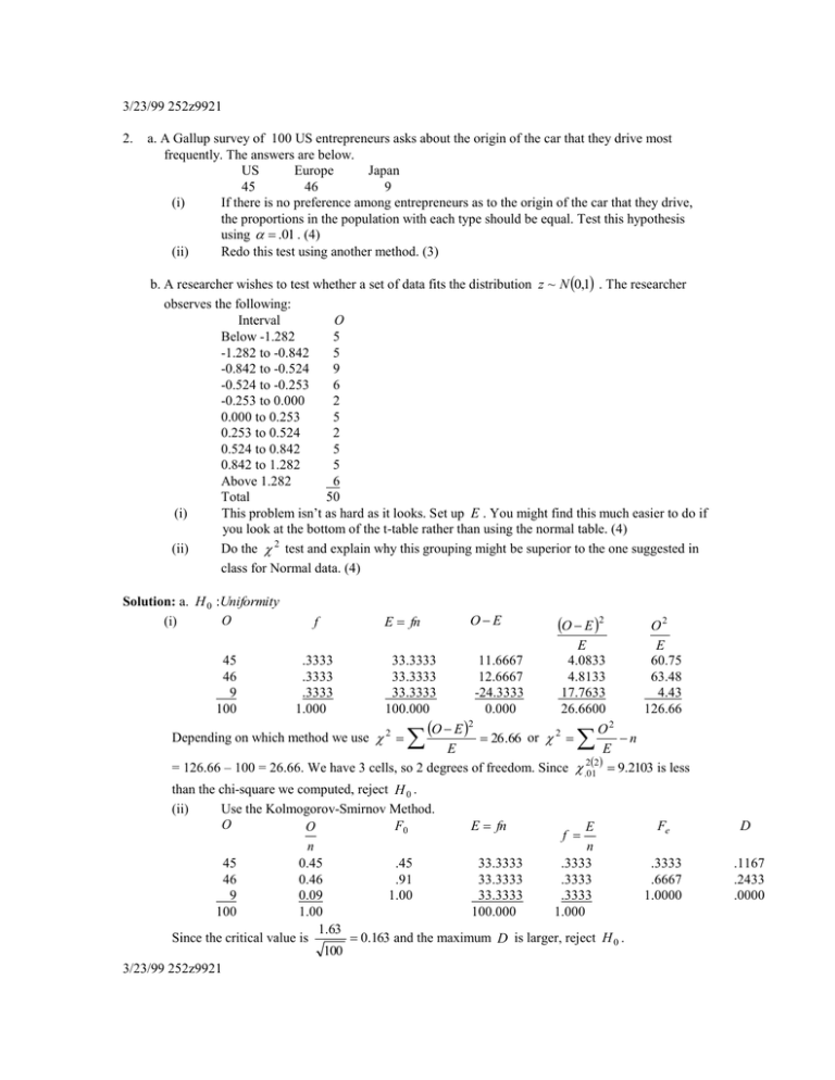
3/23/99 252z9921
2.
a. A Gallup survey of 100 US entrepreneurs asks about the origin of the car that they drive most
frequently. The answers are below.
US
Europe
Japan
45
46
9
(i)
If there is no preference among entrepreneurs as to the origin of the car that they drive,
the proportions in the population with each type should be equal. Test this hypothesis
using   .01 . (4)
(ii)
Redo this test using another method. (3)
b. A researcher wishes to test whether a set of data fits the distribution z ~ N 0,1 . The researcher
observes the following:
Interval
O
Below -1.282
5
-1.282 to -0.842
5
-0.842 to -0.524
9
-0.524 to -0.253
6
-0.253 to 0.000
2
0.000 to 0.253
5
0.253 to 0.524
2
0.524 to 0.842
5
0.842 to 1.282
5
Above 1.282
6
Total
50
(i)
This problem isn’t as hard as it looks. Set up E . You might find this much easier to do if
you look at the bottom of the t-table rather than using the normal table. (4)
(ii)
Do the  2 test and explain why this grouping might be superior to the one suggested in
class for Normal data. (4)
Solution: a. H 0 :Uniformity
O
(i)
45
46
9
100
f
.3333
.3333
.3333
1.000
OE
E  fn
33.3333
33.3333
33.3333
100.000
O  E 2
11.6667
12.6667
-24.3333
0.000
O  E 2
E
4.0833
4.8133
17.7633
26.6600
O2
E
60.75
63.48
4.43
126.66
O2
n
E
E
= 126.66 – 100 = 26.66. We have 3 cells, so 2 degrees of freedom. Since  .2012   9.2103 is less
Depending on which method we use  2 

 26 .66 or  2 

than the chi-square we computed, reject H 0 .
(ii)
Use the Kolmogorov-Smirnov Method.
O
F0
E  fn
E
O
f 
n
n
45
0.45
.45
33.3333
.3333
46
0.46
.91
33.3333
.3333
9
0.09
1.00
33.3333
.3333
100
1.00
100.000
1.000
1.63
 0.163 and the maximum D is larger, reject H 0 .
Since the critical value is
100
3/23/99 252z9921
Fe
D
.3333
.6667
1.0000
.1167
.2433
.0000
b.
(i) H 0 : N 0,1 According to the t-table 1.282  z.10 , 0.842  z .20 , 0.524  z 30 etc. So
Pz  1.282   .10 , P1.282  z  0.842   .10 etc.
O
OE
(ii)
f
E  fn
O  E 2
O2
E
E
5
.10
5
0
0.0
5.0
5
.10
5
0
0.0
5.0
9
.10
5
4
3.2
16.2
6
.10
5
1
0.2
7.2
2
.10
5
-3
1.8
0.8
5
.10
5
0
0.0
5.0
2
.10
5
-3
1.8
0.8
5
.10
5
0
0.0
5.0
6
.10
5
0
0.0
5.0
6
.10
5
1
0.2
7.2
50
1.00
50
0
7.2
57.2
We have 10 cells, so 9 degrees of freedom. Since  .2019   16.9190 is greater than the chi-square we
computed, accept H 0 .
This grouping is superior to the one shown in class because if n  50 , there will be no
items in the E column that are below 5, a condition that calls for cutting the number of cells.
7
3/23/99 252z9921
3.
a. In an ad that appeared in the Sunday Inquirer Parade Magazine (numbers slightly
modified), Astra Pharmaceuticals reported that the most frequent adverse reaction to its
heartburn drug, Prilosec, was a headache. In the reported test 32 out of 465 getting Prilosec
reported a headache, while 5 out of 73 getting a placebo reported a headache as did 15 out of
195 getting Ranitidine, another heartburn medication. Test if there is a significant difference
between these three proportions.   .05  (6)
b. Why can’t the problem above be done by the Kolmogorov-Smirnov method? (1)
c. (Extra Credit) I lied. Actually the number that received the placebo was 64 and 4 had an
adverse reaction. Why did I have to change the numbers? (2)
d. Test the hypothesis that the proportion reporting headaches with Prilosec was lower than
with Ranitidine. (4)
Solution:
a.
H 0 : Homogeneous
H 1 : Not homogeneous
O
DF   r  1 c  1  1 2  2
2 2
 .05   5.9915
pr
E
sum
pr
32 5 15
52 .070941
32 .988
5.179 13 .834 .070941
433 68 180 681 .929059
432 .012 67 .821 181 .166 .929059
sum 465 73 195 733 1.00000
sum 465 .000 73 .000 195 .000 1.00000
The proportions in rows, p r , are used with column totals to get the items in E . Note that row sums in
E are the same as in O .
O
E
32
5
15
433
68
180
733
32.988
5.179
13.834
432.012
67.821
181.166
733.000
O2
E
31.042
4.827
16.265
433.990
68.179
178.841
733.144
OE
O  E 2
-.98772
-.17872
1.16644
.98772
.17872
-1.16644
0.00000
E
.02957
.00617
.09835
.00226
.00047
.00751
.14433
O  E 2
O2
n 
E
E
 733 .144  733  0.144
Since this is less than 5.9915. do not reject H 0 .


b. The Kolmogorov-Smirnov test can only be used when the parameters are known. In tests of
independence or homogeneity, the proportions in each row and column are the parameters and are estimated
in the process of putting together E .
c. The problem is partially set up with the correct values below.
O
sum
pr
E
pr
32 4 15
51 .07044
32 .756
433 60 180
?
.?
?
sum 465 64 195 724 1.00000
sum 465 .000
We get a cell with a value below 5, which can complicate the solution.
4.508 13 .736 .07044
?
?
?
64 .000 195 .000 1.00000
8
3/23/99 252z9921
d. From Table 3 of the Syllabus Supplement:
Interval for
Confidence
Interval
p  p  z 2 sp
Difference
between
proportions
q  1 p
p  p1  p2
p1q1 p2 q 2

n1
n2
s p 
Hypotheses
Test Ratio
H 0 : p  p0
H 1 : p  p0
p 0  p 01  p 02
or p 0  0
z
p  p 0
 p
If p  0
 p 
p01q 01 p02 q 02

n1
n2
Or use s p
Critical Value
pcv  p0  z 2  p
If p0  0
 p 
p0 q 0  1 n1 
1
n2

n p  n2 p2
p0  1 1
n1  n 2
H 0 : p1  p 3
H 0 : p1  p 3  0
32
15
p1 
 .068817 , p 3 
 .076923 ,
or 

465
195
H
:
p

p
H
:
p

p

0
3
3
 1 1
 1 1
32  15
 .071212 ,   .05, z  1.645 .
p  p1  p3  .008106 , p 0 
465  195
H 0 : p  0
Same as

H 1 : p 0
 p  p 0 q 0

1
Test Ratio: z 
n1

1
n3

p  p 0
 p
.071212 .928788  1 465  1195  .02194

 .008106  0
 0.369 This is above -1.645.
.02194
or Critical Value: pcv  p0  z  p  0  1.645 .02194   .03609
p  .008106 is above this value.
or Confidence Interval: p  p  z s p where s p 
p1 q1 p 3 q 3

. ( I’ll do it if you do it!). The
n1
n3
interval includes 0. In all cases do not reject H 0 .
9
3/23/99 252z9921
4.
Two fuel additives are being tested to see whether the there is a significant difference in miles per
gallon for the two additives. The data is below.
difference
x1
x2
16.7
21.3
-4.6
17.3
18.7
-1.4
17.5
19.8
-2.3
18.2
22.1
-3.9
18.4
17.8
0.6
18.4
18.2
0.2
18.6
18.7
-0.1
19.1
21.3
-2.2
You may need some of the following numbers:   .05, x1  18.025 , s1  0.788 , n1  8,
x 2  19.738 , s 2  1.636 , n2  8, and d  1.713, s d  1.905.
a.
Test for a significant difference in miles per gallon if these are independent samples and
the underlying distribution is not Normal. (5)
b.
Test for a significant difference in miles per gallon if each line represents results for a
single vehicle and the underlying distribution is not Normal. (5)
c.
Test for a significant difference in miles per gallon if each line represents results for a
single vehicle and the underlying distribution is Normal. (5)
Solution: a. Wilcoxon-Mann-Whitney Method H 0 :  1   2
x1
r1
x2
H 1: 1   2
r2
If we correct the starred items we get the following:
16.7
17.3
17.5
1
2
3
18.2
17.8 4
5* 18.2 6*
r1
18.4 7*
18.4 8*
18.6 9
18.7
18.7
10*
11*
19.1 12
19.8
21.3
21.3
22.1
*tie
13
14*
15*
16
r2
1
2
3
5.5
7.5
7.5
9
12
47.5
4
5.5
10.5
10.5
13
14.5
14.5
16
88.5
16 17 
Check: 47 .5  88 .5  126 
2
For a 5% two-tailed test, Table 6 says that the lower
critical value is 49. The lower of the two rank sums,
W  47.5 is below this value, so reject H 0 .
10
3/23/99 252z9921
b. Wilcoxon Signed rank test for paired data. H 0 :  1   2 H 1 :  1   2 .
difference rank
If we add items with + and – signs separately, we
-4.6
8find T   31, T   5 . To check this, compute
-1.4
4T  T    31  5  36  89 . From Table 7
-2.3
62
-3.9
7with n  8 , TL   TL .025  4 , and since 5,
0.6
3+
2
0.2
2+
the smaller T is above the critical value, do not
-0.1
1reject H 0 .
-2.2
5-
c. Test of equality of means for paired data.
H 0 :   0
H :    2
or
  1   2 or  0 1

H1 :   0
H 1 :  1   2
sd 
sd
n

1.905
8
Test Ratio: t 

H 0 :  1   2  0

H 1 :  1   2  0
d  1.713, s d  1.905,
3.629025 .1089
 0.6735 , DF  n  1  7, t .7025  2.365
8
d   0  1.713  0

 2.529
sd
0.6735
This is not on the
Interval between –2.365 and +2.365.
or Critical Value: d cv   0  t s d  0  2.365 0.6735   1.593
2
d  1.713 is not on this interval.
or Confidence Interval:   d  t  2 s d  1.713  1.593  or –3.306
to –0.120. This interval does not include 0.
With all methods reject H 0 . Note that this method is more powerful than the one in c. However, it
still should not be used unless the conditions justify it.
3/23/99 252z9921
5.
The second column from the last page is repeated. (Use   .05 )
x2
21.3
18.7
19.8
22.1
17.8
18.2
18.7
21.3
You may need some of the following numbers: x 2  19 .738 , s 2  1.636 , n 2  8 .
a.
Test these data to see if the distribution is Normal. (5)
b.
Test these data to see if the distribution is Normal with a mean of 17 and a standard
deviation of 0.5. (5)
c.
Assume that the distribution is not normal and test whether these data have a median of
17.2 (3 – 5 if you use a method learned recently)
Solution: a. H 0 : N  ?, ? H 1 : Not Normal
Because the mean and standard deviation are unknown, this is a Lilliefors problem. The x values must be
x  x x  19 .738

in order From the data we find that x  19.738 and s  1.636 . t 
.This is often
s
1.636
called
z as in a K-S problem and F t  is a cumulative Normal probability computed just like F z  below.
x
t
F t 
O
O
n
Fo
D
17 .8
19 .8
21 .3
21 .3
22 .1
 1.18  0.94  0.63  0.63 0.04
.1190 .1736 .2643 .2643 .5160
1
1
1
1
1
0.95
.8289
1
0.95
.8289
1
1.44
.9251
1
0.125
0.125
.0060
18 .2
0.125
0.250
.0764
18 .7
0.125
0.375
.1107
18 .7
0.125
0.500
.2357
0.125 0.125
0.625 0.750
.1090 .0789
O  n  8
0.125 0.125
0.825 1.000
.0461 .0749
MaxD   .2357
Since the Critical
Value for   .05
is .285 , do not re ject H 0 .
b. H 0 : N 17 ,0.5
H 1 : Not N 17 ,0.5
Because the mean and standard deviation are known, this is a Kolmogorov-Smirnov problem.
x   x  17

The x values must be in order z 
.

0 .5
x
17 .8 18 .2 18 .7 18 .7 19 .8 21 .3 21 .3 22 .1
z
F z 
O
O
n
Fo
D
1.60
.9452
1
2.40
.9918
1
3.40
.9997
1
3.40
.9997
1
5.60
1.000
1
8.60
1.000
1
8.60
1.000
1
10 .20
1.000
1
O  n  8
0.125 0.125 0.125 0.125 0.125 0.125 0.125 0.125
0.125 0.250 0.375 0.500 0.625 0.750 0.825 1.000
.8202 .7418 .6247 .4997 .3750 .2500 .1250 .0000
Note that it might be better to group the repeated values together with O  2 and
MaxD   .8202
Since the Critical
Value for   .05
is .454 , reject H 0 .
O
 .25 . It would not
n
affect the results.
12
3/23/99 252z9921
c. Wilcoxon Signed rank test for paired data. H 0 :   7.2 H 1 :   7.2
The x values need not be in order (but it makes things easier). ‘difference’ below is x   .   .05 
x difference rank
So T   0, T   36 . To check this, compute
17.8
0.6
1+
18.2
1.0
2+
T  T    0  36  36  89 . From Table 7
18.7
1.5
3.5+
2
18.7
1.5
3.5+
with n  8 , TL   TL .025  4 , and since 5,
2
19.8
2.6
5+
21.3
4.1
6.5+
the smaller T is below the critical value, reject
21.3
4.1
6.5+
H0.
22.1
4.9
8
An alternative and less powerful test is the sign test. Here, note that there are 8 numbers above the median.
pvalue  2Pz  8  21  Pz  8  21  .99609   2.00391   .00782 . Since this is below the
significance level, reject H 0 .
13
3/24/99 252z9921
6.
In a wage discrimination case the following hourly wage data is reported.   .05  A Normal
distribution is assumed.
Men
Women
n1  31
n 2  17
x1  9.25
a.
b.
c.
d.
x 2  8.70
s1  0.90
s 2  1.30
Test the statement that the variance for women is greater than the variance for men. (2)
Test the statement that the variance for women is not equal to the variance for men. (2)
Test the hypothesis that men have a wage less than or equal to that of women, assuming that
the variances differ between the two populations. (6)
Repeat the test in c using the same sample means and variances, but assuming that
n1  310 and n 2  170 . (4)
H 0 :  12   22
s 2 1.30 2
16,30  1.99
Solution: a. 
is smaller than

 .05 , 22 
 2.08 . Since F  F.05
2
s1
H 1 :  12   22
0.90 2
our ratio, reject H 0 .
H 0 :  12   22
b. 
H 1 :  12   22
check is
s 22
s12
s12
s 22

0.90 2
1.30 2
 1,
s 22
s12
 2.08 . Since the first ratio is below 1, the only one we need
16,30  2.28
. Since F  F.025
is larger than our ratio, do not reject H 0 .
2
H 0 :   0
H 0 :  1   2
H 0 :  1   2  0
c. 
or 
,   .05 . See problem II for
where   1   2 or 
H 1 :   0
H 1 :  1   2
H 1 :  1   2  0
formulas.
n1  31, x1  9.25, s1  0.90 , n 2  17, x 2  8.70, s 2  1.30 , d  x1  x 2  0.55 .
s12 0.90 2

 0.02613
n1
31
s 22 1.30 2

 0.09941
n2
17
s12 s 22

 0.12554
n1 n 2
DF 
 s12 s 22 



 n1 n 2 


2
sd 
s12 s 22

 0.12554  0.3543
n1 n 2
2
2
 s12 
 s 22 
 
 
 n1 
 n2 
 
 

n1  1
n2 1

0.12554 2
0.02613 2  0.09941 2
30
 24 .609 , so use 24 degrees of freedom.
16
14
3/23/99 252z9921
t .24
05  1.711.
Test Ratio: t 
d   0 0.55  0

 1.552 This is below 1.711.
sd
0.3543
or Critical Value: d cv   0  t  2 s d  0  1.7110.3543   0.607 .
0.55 lies below this value.
or Confidence Interval:   d  t s d  0.55  1.711 0.3543   0.057
This interval includes 0. In all cases do not reject H 0 .
d.
H 0 :   0
H :    2
H 0 :  1   2  0
or  0 1
,
where   1   2 or 

H 1 :   0
H 1 :  1   2
H 1 :  1   2  0
n1  310 , x1  9.25, s1  0.90 , n 2  170 , x 2  8.70, s 2  1.30 , d  x1  x 2  0.55 .
Because of the large sample size, we can act as if the variances were known. From Table 3 in the
syllabus supplement:
Interval for
Confidence
Hypotheses
Test Ratio
Critical Value
Interval
Difference
Between Two
Means (
known)
H 0:   0
  d  z 2 d
d 
 12
n1

 22
n2
t
H1 :    0
  1   2
d  0
sd
d cv   0  z 2 d
d  x1  x 2
z .05  1.645 ,
sd 
Test Ratio: z 
s12 s 22


n1 n 2
0.90 2  1.30 2
310
170
 0.1120
d   0 0.55  0

 4.991 This is above 1.645.
sd
0.1120
or Critical Value: d cv   0  t  2 s d  0  1.645 0.1120   0.1842 .
0.55 lies above this value.
or Confidence Interval:   d  t s d  0.55  1.645 0.1120   0.366
This interval does not include 0. In all cases reject H 0 .
15
3/24/99 252z9921
IV. Computer Problem.
1. Hand in your first problem (3 – 2point penalty for not handing in).
2. Assume that your output is:
MTB > ttest mu = 30 ‘glop’;
SUBC > alt =1.
TEST OF MU=30 VS MU > 30
Variable N Mean StDev
glop
20 36.00
9.23
SE Mean T P-Value
2.06
2.91 0.0045
(Don’t do this problem unless you handed in the computer problem.)
Show how the value of t was computed from the values of the mean and standard deviation
(1)
b. Give the null hypothesis and tell, using the p-value, whether (and why) you would accept
it if   .075 . (1)
c. What would the p-value be for the following tests (2):
(i)
MTB > ttest mu = 30 ‘glop’
(ii)
MTB > ttest mu = 30 ‘glop’;
SUBC > alt = -1.
x   0 36 .00  30
s
9.23

 2.92, s x 

 2.06 .
Solution: a. t 
sx
2.06
n
20
a.
The rule on p-value: if the p-value is less than the significance level   reject the null
hypothesis; if the p-value is greater or equal than the significance level, do not reject the null
hypothesis.
 H :   30
b.  0
Since .0045 is less than the significance level (   .075 ),
 H 1 :   30
reject H 0 .
c. See diagrams.
(i) Since this is a 2-sided test, double the probability between
t and the nearest corner. Thus the p-value is 2(.0045)
= .009. (If   .075 , reject H 0 .)
(ii) This is the opposite test, so the p-value is
1 - .0045 = .9955. (If   .075 , do not reject H 0 .)
16