252y0572 12/01/05 (Page layout view!)
ECO252 QBA2 Name KEY
THIRD HOUR EXAM Hour of Class Registered
Dec 1 2005 MWF 2, MWF3, TR 12:30, TR2
I. (40 points) Do all the following (2 points each unless noted otherwise). Do not answer question ‘yes’ or
‘no’ without giving reasons.
Show your work in questions that are not multiple choice.
1. Turn in your computer problems 2 and 3 marked to show the following: (5 points, 2 point penalty for not doing.) a) In problem 2 – what is tested and what are the results? b) In problem 3 – what coefficients are significant? What is your evidence? c) In the last graph in problem 3, where is the regression line? [5]
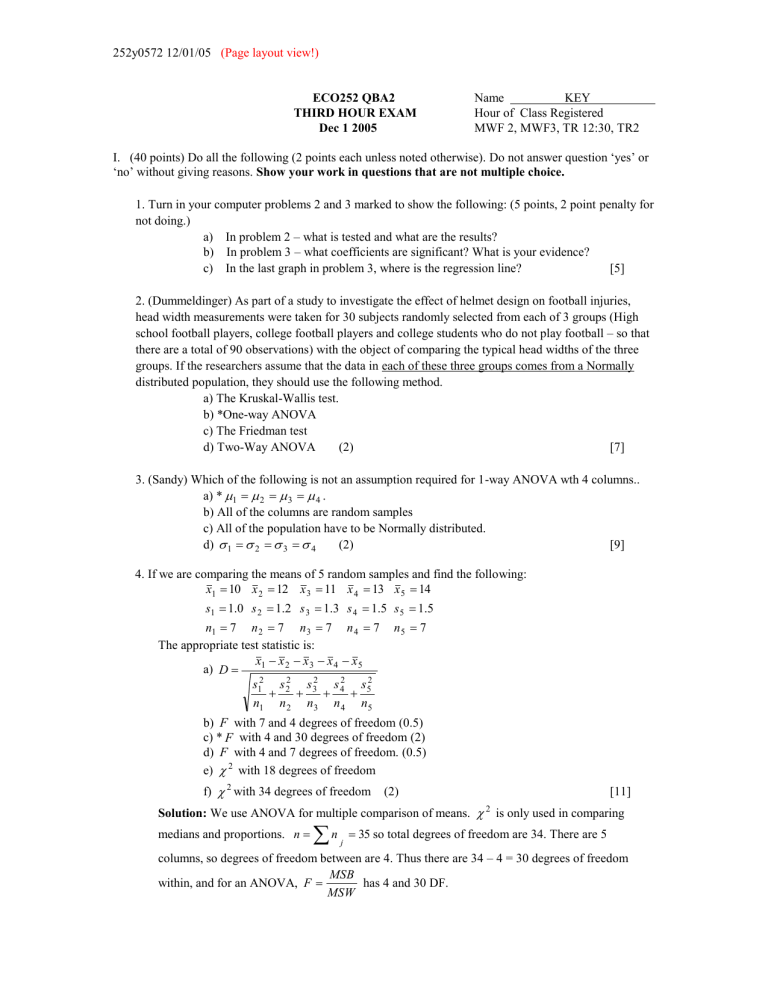
2. (Dummeldinger) As part of a study to investigate the effect of helmet design on football injuries, head width measurements were taken for 30 subjects randomly selected from each of 3 groups (High school football players, college football players and college students who do not play football – so that there are a total of 90 observations) with the object of comparing the typical head widths of the three groups. If the researchers assume that the data in each of these three groups comes from a Normally distributed population, they should use the following method. a) The Kruskal-Wallis test. b) *One-way ANOVA c) The Friedman test d) Two-Way ANOVA (2) [7]
3. (Sandy) Which of the following is not an assumption required for 1-way ANOVA wth 4 columns.. a) *

1
 
2
 
3
 
4
. b) All of the columns are random samples c) All of the population have to be Normally distributed. d)

1
 
2
 
3
 
4
(2)
4. If we are comparing the means of 5 random samples and find the following: x
1

10 x
2

12 x
3

11 x
4

13 x
5

14 s
1

1 .
0 s
2

1 .
2 s
3

1 .
3 s
4

1 .
5 s
5

1 .
5 n
1

7 n
2

7 n
3

7 n
4

7 n
5

7
The appropriate test statistic is: a) D
 x s
1
2
1

 x
2 s
2
2

 x s
3
2
3

 n
1 n
2 n
3 x
4 s
2
4 n
4
 x

5 s
5
2 n
5
[9] b) F with 7 and 4 degrees of freedom (0.5) c) * F with 4 and 30 degrees of freedom (2) d) e)
F with 4 and 7 degrees of freedom. (0.5)
 2
with 18 degrees of freedom f)
 2 with 34 degrees of freedom (2) [11]
Solution: We use ANOVA for multiple comparison of means. medians and proportions. n

 n j

35
 2
is only used in comparing so total degrees of freedom are 34. There are 5 columns, so degrees of freedom between are 4. Thus there are 34 – 4 = 30 degrees of freedom within, and for an ANOVA, F

MSB
MSW
has 4 and 30 DF.

252y0572 12/01/05 (Page layout view!)
5. If we are doing a 2-way ANOVA and find the following:
Two-way ANOVA: C5 versus C6, C7
Source DF SS MS F P
Rows 3 32.374 10.7914 2.82 0.046
Columns 2 7.861 3.9304 1.03 0.364
Interaction 6 28.999 4.8331 1.26 0.288
Error 60 229.406 3.8234
Total 71 298.639
S = 1.955 R-Sq = 23.18% R-Sq(adj) = 9.10%
The following are significant at the 5% level. a) *Differences between Row means only b) Differences between Column means only
(3) c) Both differences between Column means and Interaction d) Interaction only d) All are significant at the 5% level e) None are significant at the 5% level f) Not enough information.
Explanation: Note that only the p-value for Rows is below 5%.
[14]
6. If we do a 1-way ANOVA and find the following.
One-way ANOVA: C1, C2, C3, C4
Source DF SS MS F P
Factor 3 32.37 10.79 2.76 0.049
Error 68 266.27 3.92
Total 71 298.64
Individual 95% CIs For Mean Based on Pooled
StDev
Level N Mean StDev +---------+---------+---------+---------
C1 18 11.916 1.095 (--------*--------)
C2 18 12.436 2.195 (--------*---------)
C3 18 12.927 1.929 (--------*---------)
C4 18 13.736 2.434 (--------*---------)
+---------+---------+---------+---------
11.0 12.0 13.0 14.0
Give a 1% Tukey confidence interval (or equivalent test) for
  
3
and explain whether this shows a significant difference between these two means.
Extra Credit – do the same with a Scheffe interval. (2)
(3) [17]
Extra Credit – Do the same for an individual confidence interval for the difference and explain why it is more likely to show a significant difference than the other two. (2)
Solution: From the printout n
 m

68 , x
.
1

11 .
916 and x
.
3

12 .
927 . m

4 , s
2 
MSW

3 .
92 , n
1

18 , n
2

18 ,
First x
.
1
 x
.
3 s
1

1
 s
2 n
1 n
3

11 .
916

12 .
979


1 n
1


1 n
3

1 .
063


.

3 .
92


1
18

1
18



0 .
4356

0 .
65997 . a) Tukey Confidence Interval

1
 
3

 x

1
 x

3

 q
 m , n
 
 m
 s
2 q
 m , n
 
 m


1
 
3

1
2
 q

4 , 68

.
01

1 .
063
2


4 .
59
3 .
2456

4 .
59

2
0 .
65997

2

2

3 .
2456

1 .
063

. So
2 .
142
1 n
1

1 n
3
2

252y0572 12/01/05 (Page layout view!) b) Scheff e

Confidence Interval

1 that F

3 , 68

.
01
is between F

3 , 65

.
01

 
4
4 .
10 and

 x

1

F

3 , 70

.
01 x

3

  m

1

4 .
07 . So
F

 m

1 , n
 m
 s
1

1 n
1 n
3
F

3 , 68

.
01 must be about 4.08.
. Note

1
 m

1

F

 m

1 , n
 
3

 m


1 .
063


 
3 .
4986

F


3 , 68

0 .
65997


3

4 .
08

 
1 .
063

3 .
4986

2 .
309
. Our interval is now c) Individual Confidence Interval

1 t

 n

2 m

 t
68
.
005
 
3

2 .
650 .
Our interval is now


1
 x

1

 
3 x

3


 t

 n
2
 m
 s

1 .
063

1 n
1
2 .
650

1 n
3

0 .
65997

 
1 .
063

1 .
749
Looking back, recall that the four means were significantly different at the 5% level but not the 1% level. In this case not even the individual confidence interval shows a significant difference between the means. We know that as confidence levels go up confidence intervals have to get wider. The individual confidence interval by itself has a confidence level of 99%, but since the
Tukey and Scheffè intervals have a collective confidence level of 99%, the individual confidence intervals must have confidence levels above 99%.
7. If we do a 1-way ANOVA and find the following: (Sandy 12.50, 12.51)
One-way ANOVA:
Source DF SS MS F P
Factor ? 7.30310 1.46062 1.60
Error ? 101.358 0.913131
Total 116 108.661
The degrees of freedom for the F test are a) 4, 100 b) 5, 111 c) 4, 111 d) 5, 115. e) 5, 116 f) 4, 115
(2)
Explanation: 7.30310/5 = 1.46062. 101.358/111 = 0.913135. 5 + 111 = 116.
[19]
8. If we do a 1-way ANOVA and assume that your answer in 7 is correct, pick an appropriate value for
F with a 10% significance level from the table and explain your results. (2) [21]
Solution:
F
From the F table - between 1.99 and 2.00;

4 , 115

.
10
F

.
10
F
5 , 115


4 , 100
.
10

is 2.00; F

5 , 111
.
10

is between 1.89 and 1.91;
is between 1.89 and 1.91; F

5 , 116
.
10

F

4 , 111
.
10

is
is between 1.89 and 1.91;
is between 1.99 and 2.00. In any case, the computed value of F is below the table value, so we cannot reject the null hypothesis of equal factor means.
3

252y0572 12/01/05 (Page layout view!)
9. If we do a simple regression and find the following: (Sandy 13.1, 13.2)
If we do a simple regression and find the following: (Sandy 13.1, 13.2)
 xy

1200 , 5 y

,
 x
2 
500 .
The predicted value of a) 5.2 x

, 10 , n

10 y when x

4 is: b) *7.2 c) 8.6 d) 9.6 e) Answer cant’t be obtained with information given.
Explanation:
SSx
Sxy b
1


 x
2  n x

 xy
 n x y
Sxy
SSx


 x xy
2
2



 b
0
 y
 b
1 x
 x
10


 n n x x n x y
2

500
1200


2 .
80

5
10

10
 
2

?
10
700
250



4
5

 y
500

2 .
80


 n
1200 y
250



10
500
?
250

So the equation is

700
Y
ˆ
10

Y
ˆ  
4

2 .
8

7 .
2

4

2 .
8 X
(4) [25]
and if x

4 ,
10. Assume the following data: x y
7
9
5
-2
-6
-1
8 -9
29 -18
Find the following. Show your work!
 x
2
,
 xy , R
2
Row x y x
2 y
2 xy
1 7 -2 49 4 -14
2 9 -6 81 36 -54
3 5 -1 25 1 -5
4 8 -9 64 81 -72
29 -18 219 122 -145 Starred quantities must be positive.
x

 n x

29
4

7 .
25 y

 n y


18
4
 
4 .
5
(4)
SST
SSx
Sxy b
1



SSy

 y
2  n y
 x
2  n x
2 
219
2


 xy
 n x y
Sxy
SSx


 x xy
2




145 n x y n x
2



4

7 .
25


122
4

7 .
25
 
14
8 .
75

.
5
4
 
2

2 
219


1 .
657


122 81
210 .
25

145


130


.
5
41

*
8 .
75 *

14 .
5
SSR
 b
1
Sxy
 
1 .
657 (

14 .
5 )

24 .
0265 * So R
2
R
2

SSR

SST
24 .
0265
41

.
5860 or

 
SSx
2
  




14 .
5
8 .
75

2
 

210 .
25
358 .
75

.
5861 This must be between zero and one.
[29]
4

252y0572 12/01/05 (Page layout view!)
11. The coefficient of determination is defined as a) Total (squared) variation in b) *Explained variation in y divided by the explained variation. y divided by the total (squared) variation in y c) Unexplained variation in y divided by the total (squared) variation in y . d) Sum of the explained and unexplained variation in y divided by the total variation in y . [31]
————— 11/28/2005 8:40:25 PM ————————————————————
Welcome to Minitab, press F1 for help.
MTB > Regress c1 1 c2;
SUBC> Constant;
SUBC> Brief 3.
Regression Analysis: Y versus X
The regression equation is
Y = 4.53 + 10.2 X
Predictor Coef SE Coef T P
Constant 4.531 7.217 0.63 0.548
X 10.198 1.256 8.12 0.000
Analysis of Variance
Source DF SS MS F P
Regression 1 3993.5 3993.5 65.89 0.000
Residual Error 8 484.9 60.6
Total 9 4478.4
Obs X Y Y
ˆ
1 2.00 22.00 24.93
2 7.00 68.00 75.92
3 5.00 68.00 55.52
4 8.00 96.00 86.11
5 5.00 46.00 55.52
6 8.00 80.00 86.11
7 5.00 52.00 55.52
8 3.00 38.00 35.12
9 7.00 78.00 75.92
10 4.00 48.00 45.32
 y

596 ,
 x

54 and
 x
2 
330
12. From the computer output above, find the following: a) R
2
(2) b) s e
(2) c) A 90% confidence interval for

1
(2) d) A 90% prediction interval for Y when X

5 .
(3) [40]
General Comment: Note that the table giving the regression equation and the ANOVA are something that you should understand. The values b
0

4 .
531 and b
1

10 .
198 appear there. To their right are s b 0

7 .
217 and s b 1

1 .
256 . These are used in the t ratios that appear next. But you should be able to ignore them and note that because the p-value for the constant is above any significance level that you might use, the constant is not significant. For the coefficient of X the p-value is below any significance level that you might use, so the coefficient is highly significant. a) R
2
Solution: The ANOVA table says
SSE

SST

SSR

484 .
9 .
SSR

3993 .
5 , SST

4478 .
4 and
R
2 
SSR

SST
3993 .
5
4478 .
4

.
8917
5

252y0572 12/01/05 (Page layout view!) b) s e
Solution: s e

60 .
6125 s
2 e

SSE n

2

7 .
7854

  
2 n

2

SS y
 b
2
SS x n

2

SST

SSR n

2

484 .
9
8

60 .
6125
c) A 90% interval for

1
. The regression output has
Predictor Coef SE Coef T P
Constant 4.531 7.217 0.63 0.548
X 10.198 1.256 8.12 0.000 df

1
 n
 b
1

2

8 t
.
05

1 .
860 s b
1


1 .
860
10 .
198

1 .
860

1 .
256


10 .
198

2 .
336 d) A 90% prediction interval for
Y
0

Y
ˆ
0
 t s
Y
, where s
Y
2  s e
2

 n
Y when
1


X
0

SS
X
X


2 x
5 .

Solution: The Confidence Interval is
1


. The table above says that if x

5 ,
Y
ˆ s
Y
2


55 .
52 s e
2


1 n
.

X


SS x
X x x


0 n

2

54
10

1



5 .
4 SSx
60 .
6125

1
10

 x
2  n x
38 .
4
2

5

5 .
4

2

330

10
 
2

1


60 .
6125

330


1 .
1

291 .
60
0 .
00467



38 .
4 .
66 .
9263 s
Y
ˆ

66 .
9263

8 .
18085

Y
0

55 .
52

1 .
860

8 .
18085


55 .
52

15 .
22
I won’t comment on the computer assignments except to say that there was a table in the second assignment like that in question 5. There were 3 tests here and you should have said what they were and stated the meaning of the specific p-values. For the regression see the general comment on question 12.
6