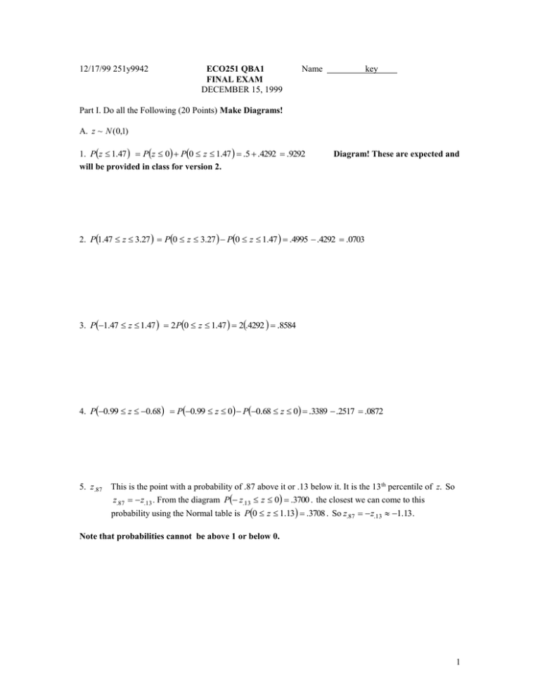
12/17/99 251y9942
ECO251 QBA1
FINAL EXAM
DECEMBER 15, 1999
Name
key
Part I. Do all the Following (20 Points) Make Diagrams!
A. z ~ N (0,1)
1. Pz  1.47   Pz  0  P0  z  1.47   .5  .4292  .9292
will be provided in class for version 2.
Diagram! These are expected and
2. P1.47  z  3.27   P0  z  3.27   P0  z  1.47   .4995  .4292  .0703
3. P1.47  z  1.47   2P0  z  1.47   2.4292   .8584
4. P0.99  z  0.68   P0.99  z  0  P0.68  z  0  .3389  .2517  .0872
5. z .87 This is the point with a probability of .87 above it or .13 below it. It is the 13 th percentile of z. So
z.87   z.13 . From the diagram P z.13  z  0  .3700 . the closest we can come to this
probability using the Normal table is P0  z  1.13   .3708 . So z.87   z.13  1.13.
Note that probabilities cannot be above 1 or below 0.
1
12/17/99 251y9942
B. x ~ N 1.5, 3 . As usual, people made diagrams of x with zero in the middle. Make up your mind!
If you are diagramming x , put the mean in the middle; if you are diagramming z put zero in the
middle.
1.47  1.5 

1. Px  1.47   P z 
  Pz  0.01  Pz  0  P 0.01  z  0  .5  .0040  .4960
3


Remember z 
x

.
3.27  1.5 
 1.47  1.5
z
2. P1.47  x  3.27   P
  P 0.01  z  0.59 
3
3


 P 0.01  z  0  P0  z  0.59   .0040  .2224  .2264
1.47  1.5 
  1.47  1.5
z
3. P1.47  x  1.47   P
  P 0.99  z  0.01
3
3


 P0.99  z  0  P0.01  z  0  .3389  .0040  .3349
 0.68  1.5 
  0.99  1.5
z
4. P0.99  x  0.68   P
  P 0.83  z  0.73 
3
3


 P0.83  z  0  P0.73  z  0  .2967  .2673  .0294
5. x.87 This is the point with a probability of .87 above it or .13 below it. It is the 13 th percentile of x .
Because it is below the 50th percentile, which is the mean for the Normal distribution, the point we
want will be below 1.5. On the previous page we found z.87   z.13  1.13. So x.87    z.87
 1.5  1.133  1.89.
 1.89  1.5 

To check to see if this is correct: Px  1.89   P z 
  Pz  1.13 
3


 Pz  0  P1.13  z  0  .5  .3708  .8708  .87
2
12/17/99 251y9942
II. (4 points-2 point penalty for not trying .) Show your work!
A manufacturer of printheads investigates the amount of time before a printhead fails. The
data for a sample of 8(in millions of characters)are below.
x
1.5
1.4
1.2
1.6
2.1
1.3
1.4
1.5
Compute the sample standard deviation, s . Show your work. (4)
Solution:
Printhead lives
x
x2
1
1.5
2.25
2
1.4
1.96
3
1.2
1.44
4
1.6
2.56
5
2.1
4.41
6
1.3
1.69
7
1.4
1.96
8
1.5
2.25
12.0 18.52
 x  12  1.50
x
n
8
s x2
s x  0.0742857  0.27255
x

18 .52  81.50 2 0.52

 0.0742857
n 1
7
7


s
0.27255
 sx  x 
 0.0963624 

n
8


2
 nx 2

3
12/17/99 251y9942
III. Do at least 4 of the following 7 Problems (at least 12 each) (or do sections adding to at least 48 points Anything extra you do helps, and grades wrap around) . Show your work!
1. Using the sample standard deviation from the sample of 8 on the previous page. (Assume that the
parent population is Normal.)
a. Compute a 95% confidence interval for the mean time before a printhead fails. (4)
b. Compute a 95% confidence interval for the mean time before a printhead fails assuming that the
sample of 8 was taken from a batch of 80 printheads. (4)
c. Compute a 95% confidence interval for the mean time before a printhead fails assuming that the
population standard deviation is known to be 1.40 and the population is very large. Sample size is
still 8. (4)
Solution: From the previous page x  1.50 , s x2  0.0742857 , s x  0.27255 , s x 
sx
 0.0963624 .
n
a) For a) and b) population variance is unknown, so we must use t instead of z. The general formula for a
confidence interval is   x  tn1 s x . Here the degrees of freedom are n  1  8  1  7 and since the
2
7
confidence level is 95%, 1    .95 or   .05 . Also tn1  t .025
 2.365 .
2
From the previous problem. s x  0.0742857  0.27255
sx 
sx

0.27255
n
 0.0963624
8
Putting this all together   x  tn1 s x  1.5  2.365 0.0963624   1.5  0.2279 or 1.27 to 1.73. More
formally, P1.27    1.73   .95
2
b) The population size, N  80 , is less than 20 times the sample size n  8 so s x 
N n
N 1
sx
n
80  8

 0.0963624 0.9546687   0.091994 and   x  tn1 s x
2
80  1
8
 1.5  2.365 0.091994   1.5  0.2176 or 1.28 to 1.72.
0.27255
c) This time  x  1.40 is known, so we can replace t with z   z .025  1.960 .  x 
2
x
n

1.40
 0.4950
8
and   x  z   x  1.5  1.960 0.4950   1.5  0.9702 or 0.53 to 2.47.
2
4
12/17/99 251y9942
2. The Freshman class at Chest Wester University has SAT Math scores that are normally distributed with a
mean of 490 and a standard deviation of 60.
a. What is the probability that a class of 36 will have a mean score below 476? (3)
b. What is the probability that a person randomly picked from the Freshman class will have a score
below 476? (2)
c. Assuming that the class is quite large, what is the probability that 10 people picked randomly from
the Freshman class will all have a score below 476? (2)
d. What score would you have to have to be at the 95 th percentile of this class? (3)
e. Create a symmetrical interval around 490 that contains 70% of the Freshman math scores. (2).
f. What is the probability that, if I pick 10 people from the Freshman class, 8 or more of them will have
scores above 490? (2)
Solution: From the problem statement x ~ N 490 , 60  , i.e.   490,   60 and for the sample mean,
x 
x
n

60
 10 .
36
476  490 

a) Px  476   P z 
  Pz  1.40   Pz  0   P 1.40  z  0  .5  .4192  .0808
10


476  490 

b) Px  476   P z 
  Pz  0.23   Pz  0  P 0.23  z  0  .5  .0910  .4090
60


c) Binomial probability of 10 out of 10 when p  .4090 is .4090 10  1.3099 10 4  .00013099 .
d) From the t table z .05  1.645 . So x.05    z.05  490  1.645 60   538 .70.
e) From the t table z .15  1.036 . So x    z  490  1.03660  490  62.16 or 427.84 to
552.16.
f) Since the probability of being above the mean is .5, this is a binomial problem with n  10, p  .5.
Px  8  1  Px  7  1  .94531  .05469 .
5
12/17/99 251y9942
3. 10% of the patients at my hospital are dissatisfied with their experience. Last Monday 14 patients were
discharged. All filled out surveys.
a. In this group of 14, what was the mean and variance of the number that were dissatisfied? (2)
b. What was the probability that over half of those discharged were dissatisfied? (2)
c. What was the probability that at least one was dissatisfied? (2)
d. If, instead, 55% of my patients were dissatisfied, what is the probability that at least half of the
group of 14 would be dissatisfied? (2)
e. If 55% of my patients were dissatisfied, what is the chance that at least one of the group of 14
would be dissatisfied? (2)
f. If 55% of my patients were dissatisfied, and 180 were discharged in one day, what is the
probability that at least half would be dissatisfied? (Don’t answer yet!)
(i) Can this problem be done using the Poisson distribution? Why? If it can be done using
the Poisson distribution, do it! (2)
(ii) Can this problem be done using the Normal distribution? Why? If it can be done using
the Normal distribution, do it! (3)
Solution: Binomial p  .10, n  14.
a)   np  14.10   1.4.  2  npq  1.4.90  1.26
b) Px  7  1  Px  7  1  .99998  .00002
c) Px  1  1  Px  0  1  .22877  .77123
d) 7 or more successes when
p  .55, n  14
is 7 or fewer failures when the probability of failure
is .45. Px  7  .74136 .
e) The probability of one being satisfied is .45. The probability that all are satisfied is
.45 14  1.13962 10 5 . So the probability that at least one is not satisfied is
1  .45 14  1  1.13962 10 5  .999986 . To use the table to do this, reason that if at least one is
not satisfied, not all are satisfied. Look up Px  14   Px  13   .99989 for p  .45, n  14 .
f) (i) You cannot use the Poisson distribution since
n 180

 327 .27 is below 500.
p .55
(ii) You can use the Normal distribution because   np  180 .55   99  5 and
nq  180  99  81  5 .  2  npq  99.45  44.55. Without continuity correction

90  99 
  Pz  1.20   Pz  0  P 1.20  z  0  .5  .3849  .8849 .
Px  90   P z 
44 .55 

Or with the continuity correction,

89 .5  99 
  Pz  1.27   Pz  0  P 1.27  z  0  .5  .3980  .8980
Px  89 .5  P z 

44 .55 

6
12/17/99 251y9942
4. n  9 observations of the velocity x  that at which a ball is thrown and the distance  y  that it is hit are
reported below.(Ab p9-34)
Note that all the sums are computed for you. Do not compute any other sums when doing this problem. Find
the covariance and correlation between the velocity of the pitch and the distance the ball goes. (7)
a) Interpret the correlation. What does this mean about the likelihood that a given hit will be a
home run? (2)
b) A sample is taken in another stadium. It is identical to the numbers shown here except all the
distances are 5 feet longer. What would the new covariance and correlation be? (3)
x
x2
y
xy
y2
328
20
107584
400
6560
336
30
112896
900 10080
341
40
116281
1600 13640
349
50
121801
2500 17450
357
60
127449
3600 21420
364
70
132496
4900 25480
371
80
137641
6400 29680
379
90
143641
8100 34110
389 100
151321
10000 38900
3214 540
1151110
38400 197320
Solution:
 xy  197320
sxy 
x

y
 y  3214  357 .11111 ,
x
n

n
y
540
 60 , sx2 
9
 xy  nx y  197320  960 357 .11111   4480  560
n 1
x
2
 nx
n 1
9 1
2

8
38400  960 2 6000

 750 ( s x 
8
8
750  27 .38613 )
9
1151110  9357 .11111 2 3354 .8961

 419 .36201
n 1
8
8
s xy
560
( s y  419.36201  20.47833 )
rxy 

 .9970
sx s y
750 419 .36201
s 2y 
2
 ny 2

It is still true that a correlation cannot be above 1 or below –1!
Note: Because of a misprint of the x 2 sum, most people taking this version of the exam will have gotten a
correlation above 1. ( They got sx2  300 , s x  17.3205 , rxy  1.58 .) This should have been reported to me
and reported in the interpretation below. Grades were adjusted to compensate for this error.
a) The positive sign of rxy , the sample correlation, indicates that x and y tend to move closely
together. If we square rxy , we get approximately .994, which on a zero to one scale indicates a
very strong relationship. This means that the faster the pitch, the more likely that a hit will be a
home run.
b) We are leaving x alone, but replacing y by y  3 . From the syllabus supplement and the
outline if w  ax  b  1x  0 and v  cy  d  y  3 so that a  1 and b  0 , c  1 and d  3 ,
 wv  Cov(ax  b, cy  d )  acCov( x, y)  11560   560 . (Unchanged)
Corrw, v  rwv  signacrxy  sign11.9970  sign 1.9970  .9970 (Unchanged)
7
12/17/99 251y9942
5. a) Two events A1 and B1 are independent. P A1   .4 , PB1   .2 . Find the following.
(i) Can A1 and B1 be mutually exclusive? Why? (1)
(ii) P A1  B1  (1)


(iii) P A1 B 1 (1)
(iv) P A1  B1  (2)
b) Now assume that A1 is independent of B1 , B 2 and B 3 , A2 is independent of B1 , B 2 and B 3 ,
and A3 is independent of B1 , B 2 and B 3 . P A2   .3 , PB2   .3 , that A1 , A2 and A3 are mutually
exclusive and collectively exhaustive relative to one another, and that B1 , B 2 and B 3 are mutually
exclusive and collectively exhaustive relative to one another. Fill in the joint probability table below.(3)
B1 B 2 B3
A1 .... .... .... 


A2 .... .... .... 
A3 .... .... .... 


c) Now assume that a machine has two components. A1 is the probability that component 1 fails in
period 1, A2 is the probability that component 1 fails in period 2 and A3 is the probability that
component 1 fails in period 3. B1 is the probability that component 2 fails in period 1, B 2 is the
probability that component 2 fails in period 2 and B 3 is the probability that component 2 fails in
period 3.
Assume that the machine works as long as any one component works. (i) If event A1  B1 occurs,
During which period will the machine go down? (1) What about event A1  B2 ? (1) Find the probability
that the machine goes down in period 1(1), period 2 (2) and period 3 (2). Use the joint probability table
that you created in b).
Solution: a) Two events A1 and B1 are independent. P A1   .4 , PB1   .2 . .
(i) A1 and B1 cannot be mutually exclusive? Briefly, no two possible events can be both. If A1
and B1 are mutually exclusive P A1  B1   0 but see (ii) below.
(ii) If A1 and B1 are independent P A1  B1   P A1 PB1   .4.2  .08 .


(iii) If A1 and B1 are independent, by definition P A1 B1  P A1   .4
(iv) P A1  B1   P A1   PB1   P A1  B1   .4  .2  .08  .52
b) Because A1 , A2 and A3 are mutually exclusive and collectively exhaustive relative to one another, and
P A1   .4 and P A2   .3 , P A3   1  P A1   P A2   1  .4  .3  .3 . Similarly, if B1 , B 2 and B 3 are
mutually exclusive and collectively exhaustive relative to one another and PB1   .2 and PB2   .3 ,
then PB3   .5 . Because of the independence assumption, the numbers in the joint probability table will be
B1 B2 B3

A1 .08 .12 .20  .4


the product of the marginal probabilities. A2 .06 .09 .15  .3 .
A3 .06 .09 .15  .3


.2 .3 .5
1.0
8
12/17/99 251y9942
c) Because the machine works as long as the longest lived component works, the event A1  B1 downs the
machine in period 1, but the event A1  B2 downs the machine in period 2. So the various joint events
down the machine as follows:
Event
A1  B1
A1  B2
Period Probability
1
.08
2
.12
3
.20
A1  B3
2
.06
A2  B1
2
.09
A2  B2
3
.15
A2  B3
3
.06
A3  B1
3
.09
A3  B2
3
.15
A3  B3
So PPeriod 1  P A1  B1   .08
PPeriod 2  P A1  B2   P A2  B1   P A2  B2   .12  .06  .09  .27
or PPeriod 2  1  PPeriod 1  PPeriod 3  1  .08  .65  .27
PPeriod 3  P A1  B3   P A2  B3   P A3  B1   P A3  B2   P A3  B3 
 .20  .15  .06  .09  .15  .65
or PPeriod 3  P A3  B3   P A3   PB3   P A3  B3   .3  .5  .15  .65
Note that, since no component lasts beyond period 3, these three probabilities must add to one.
9
12/17/99 251y9942
6.
a. A professor has a pool of 20 multiple choice questions involving discrete probability
distributions. Four of these questions involve the Hypergeometric distribution. Assume that he
picks 6 questions at random to put on a quiz. What is the probability that at least one concerns the
Hypergeometric distribution? (3)
b. What is the mean and variance of the number of questions that concern the Hypergeometric
distribution on the above quiz? (2)
c. What would the answer to the above be if the pool of questions contained over 120 questions but
the proportion that involve the Hypergeometric distribution was the same as in a)? Do not use the
same distribution as you used in a).(2)
d. A student has not studied for the above six-question quiz. Each multiple-choice question has
five answers and she picks one randomly. What is the chance that she will get at least four right?
(2)
e. A student is extremely well-prepared for an exam. Nevertheless she knows that since she is tired
she will make an average of .1 mistake per page. The exam is 7 pages. What is the probability that
she will turn in a perfect exam? (2)
f. In the exam in e, the professor takes off 2 points for each mistake. What is the variance of the
number of points he will take off on her exam? (2)
Solution: a) Hypergeometric N  20, M  4, n  6. Px  
Px  1  1  P0  1 
C04C616
C620
C xM C nNxM
C nN
. p
M
4

 .2 q  1  p  .8.
N
20
16!
16  15  14  13  12  11
10!6!
6  5  4  3  2 1
 1
 1
 1  .2066  .7934
20!
20  19  18  17  16  15
14!64!
6  5  4  3  2 1
1
N n
20  6
14
0.96   .7074
npq 
6.2.8 
N 1
20  1
19
c) Since there was some vagueness in this question, either of the two following answers were
accepted – 3 points was given for an answer to both. Binomial p  .2, n  6. The rule of
thumb for replacing the Hypergeometric by the binomial is that the population should be 20 times
the sample.
(i) From the binomial table, p  .2, n  6. Px  1  1  P0  1  .26214  .73786
b)   np  6.2  1.2,  2 
(ii)   np  6.2  1.2,  2  npq  6.2.8  .96
d) p  .2, n  6. Px  4  1  Px  3  1  .98304  .01696
e) Poisson m  0.17  0.7 P0  .49659
f) Poisson m  0.7   2 Since Varax  a 2Varx , Var2x  22Varx  40.7  2.8 .
Note that it is still true that probabilities cannot be above 1 or below 0.
10
12/17/99 251y9942
7. A soft drink machine dispenses an amount of beverage that is distributed according to the continuous
Uniform distribution between 6.5 and 7.5 oz.
a. What is the mean and variance of the number of ounces dispensed by the machine. (2)
b. What is the probability that a given drink will contain more than 7.1 oz.? (2)
c. What is the probability that a given drink will contain between 6.3 and 7 oz? (1)
d. Using the results of a) and your knowledge of the distribution of the sample mean, if the
machine is tested by being used 100 times, what is the mean and variance of x , the average
amount of soft drink dispensed? (2)
e. What is the probability that the sample mean in d) will exceed 7.02 oz.? (3)
f. What is the probability that the total amount of liquid dispensed in 100 uses will exceed 700 oz.?
(2) 710 oz.? (2)
Solution: a)  
 
c  d 6.5  7.5

 7.0
2
2
0.08333  0.28878
2 
d  c2

12

7.5  6.52
12

1
 0.08333
12
7.5  7.1
 .4000 Make a diagram.
7.5  6.5
7.0  6.5
 .50000 .
c) P6.3  x  7.0  
7.5  6.5
b) Px  7.1 
d) x  N  ,  x  and  x 
2
x
n

0.0833
 0.028868 or   7.0 and
100
0.08333
 .0008333 (The mean and variance come from a) )
100
7.02  7.0 

e) Px  7.02   P z 
  Pz  0.69   Pz  0  P0  z  0.69   .5  .2549  .2451
.028868 

f) (i) If 700 oz. are dispensed in 100 uses, the mean amount dispensed is 7.0. Since 7.0 is the mean
and median of the distribution Px  7.0  .5 .
(ii) If 710 oz. are dispensed in 100 uses, the mean amount dispensed is 7.1. Px  7.1
 x2 
n

7.1  7.0 

 P z 
  Pz  3.46   Pz  0  P0  z  3.46   .5  .4997  .0003
.028868 

11
12/17/99 251y9942
IV. Extra Credit
1. Find P5  x  10  when p  .07 and n  200 using the normal distribution with a continuity
correction. According to the criterion you were taught, was the correction needed? Explain. Try
the problem without the correction. How much difference did it make? (5)
2. (p 84)In a hockey league the length of time elapsed before a winning goal is scored has an
exponential distribution with a mean of 8 minutes. What is the probability that the winning goal is
scored in 3 minutes or less? (2)
3. If a winning goal is not scored within 20 minutes, the game will be a tie. What is the probability
of this happening? (2)
Solution: 1) Binomial P5  x  10  when p  .07, n  200 ., q  1  p  .93 . To use the
Normal distribution we require   np  200 .07   14  5 and nq  n  np  200 14  186  5. In
addition  2  npq  200.07.93  13.02 . Since the variance is above 9, a continuity correction
is supposedly not needed.
Without the continuity correction
 5  14
10  14 
  P 2.49  z  1.11  .4936  .3665  .1271 .
P5  x  10   P
z

13 .02 
 13 .02
With the continuity correction
 4.5  14
10 .5  14 
  P 2.63  z  0.97   .4957  .3340  .1617
P4.5  x  10 .5  P
z

13 .02 
 13 .02
The error is over .03, about 1/5 of the result. This looks fairly large to me.
1
2) The Exponential distribution has F x 1  e cx where   . For these problems
c
1 1
c    0.125 .
 8
Px  3  F 3  1  e 0.1253  1  e 0.375  1  .6873  .31271.


3) Px  20  1  Px  20  1  F 20  1  1  e 0.12520  e 2.5  .082085.
12