advertisement
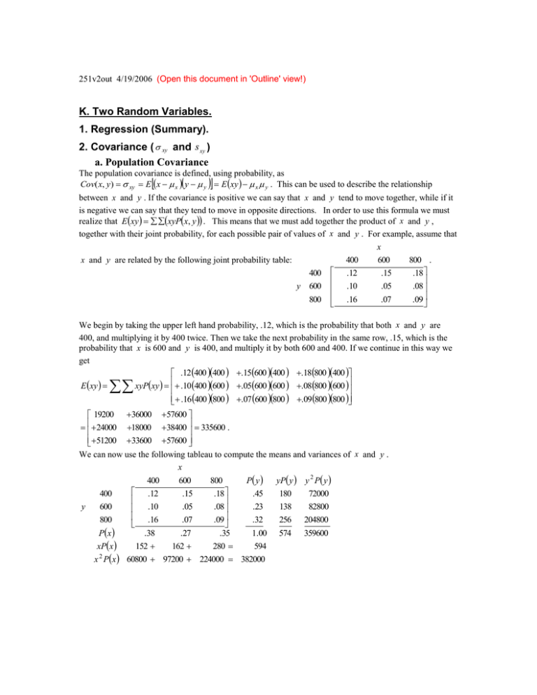
251v2out 4/19/2006 (Open this document in 'Outline' view!) K. Two Random Variables. 1. Regression (Summary). 2. Covariance ( xy and s xy ) a. Population Covariance The population covariance is defined, using probability, as Cov( x, y ) xy E x x y y E xy x y . This can be used to describe the relationship between x and y . If the covariance is positive we can say that x and y tend to move together, while if it is negative we can say that they tend to move in opposite directions. In order to use this formula we must realize that E xy xyPx, y . This means that we must add together the product of x and y , together with their joint probability, for each possible pair of values of x and y . For example, assume that x x and y are related by the following joint probability table: 400 y 600 800 400 .12 600 .15 .10 .05 .16 .07 800 . .18 .08 .09 We begin by taking the upper left hand probability, .12, which is the probability that both x and y are 400, and multiplying it by 400 twice. Then we take the next probability in the same row, .15, which is the probability that x is 600 and y is 400, and multiply it by both 600 and 400. If we continue in this way we get .12 400 400 .15600 400 .18800 400 E xy xyPxy .10 400 600 .05600 600 .08800 600 .16 400 800 .07 600 800 .09 800 800 19200 36000 57600 24000 18000 38400 335600 . 51200 33600 57600 We can now use the following tableau to compute the means and variances of x and y . x 400 600 800 P y yP y y 2 P y .12 400 .15 .18 .45 180 72000 y 600 .05 .08 .23 138 82800 .10 .16 800 .07 .09 .32 256 204800 Px .38 .27 .35 1.00 574 359600 xPx 152 162 280 594 2 x Px 60800 97200 224000 382000 Px 1 (a check), E x xPx 594 , E x x P y 1 , E y yP y 574 and E y y P y 359600 2 To summarize x 2 2 Px 382000 , 2 y We will need the variances below. To complete what we have done, write xy Covxy Exy x y 335600 594574 5356 b. The Sample Covariance The sample covariance is much easier to compute, the formula being s xy x x y y xy nx y . n 1 n 1 For example, assume that we have data on income ( x ) and savings ( y )(in thousands) for 5 families. x y x2 y2 xy 1 2 3 4 5 1.9 12.4 6.4 7.0 7.0 0.0 0.9 0.4 1.2 0.3 3.61 153.76 40.96 49.00 49.00 0.00 0.81 0.16 1.44 0.09 0.00 11.16 2.56 8.40 2.10 Sum 34.7 2.8 296.33 2.50 24.22 Family Then x s x2 34 .7 2 .8 6.94 and y 0.56 . 5 5 x 2 nx 2 n 1 y 296 .33 56.94 2 13 .878 , 4 2.50 50.56 2 0.2330 and since n 1 4 24.22 56.94 0.56 xy 24 .22 , s xy 1.197 . 5 1 The positive sign of s xy , the sample covariance, indicates that x and y tend to move together. s 2y 2 ny 2 2 3. The Correlation Coefficient ( xy and rxy ) The size of a covariance is relatively meaningless; to judge the strength of the relationship between x and y we need to compute the correlation, which is found by dividing the covariance by the standard deviations of x and y. a. Population Correlation. For the population covariance, recall from above that x2 E x 2 x2 382000 594 2 29164 and y2 E y 2 y2 359600 5742 30124 . So that xy xy x y 5356 5356 0.181 . 170 .77 173 .56 29164 30124 The correlation must always be between positive and negative 1 1.0 1.0 . A correlation close to zero is called weak. A correlation that is close to one in absolute value is called strong. (Actually statisticians prefer to look at the value of the correlation squared.) A strong positive correlation indicates that x and y have a relationship that is close to a straight line with a positive slope. A strong negative correlation means that the relationship approximates a straight line with a negative slope. Unfortunately, the correlation only indicates linear relationships; a nonlinear relationship that is obvious on a graph may give a zero correlation. b. Sample Correlation. Recall that s xy 1.197 , s x2 13 .878 , and s 2y 0.2330 . If we divide the correlation by the two standard deviations, we find that rxy s xy sx s y 1.197 0.6657 . 13 .878 0.2330 4. Functions of Two Random Variables. Cov(ax b, cy d ) acCov( x, y) and if w ax b and v cy d , wv signac xy or Corr (ax b, cy d ) (sign(ac))Corr ( x, y) , where signac has the value 1 or 1 depending on whether the product of a and c is negative or positive. 5. Sums of Random Variables. a. Ex y Ex E y and Var x y x2 y2 2 xy Var x Var y 2Covx, y b. Independence. 3 (i) Definition. Px, y Px P y (ii) Consequences If x and y are independent, E xy E x E y , Covx, y 0 , xy 0 and Varx y Varx Var y . c. If a, c and d are constants, Var(ax cy) a 2Var( x) c 2Var( y) 2acCov( x, y) . This and a. imply that Eax cy d aEx cE y d and Var(ax cy d ) a 2Var( x) c 2Var( y) 2acCov( x, y) d. Application to portfolio analysis If R P1 R1 P2 R2 and P1 P2 1 , then E R P1 E R1 P2 E R2 and VarR P12VarR1 P22VarR2 2P1 P2CovR1 , R2 . Variance is usually considered a measure of risk, though actually, the best measure of risk is probably the coefficient of variation, the standard deviation divided by the mean, in this case C R . E R The remainder of this material can be found in the Supplement in the document 251var2. You can get a slightly expanded version of this at 251varmin . 4
