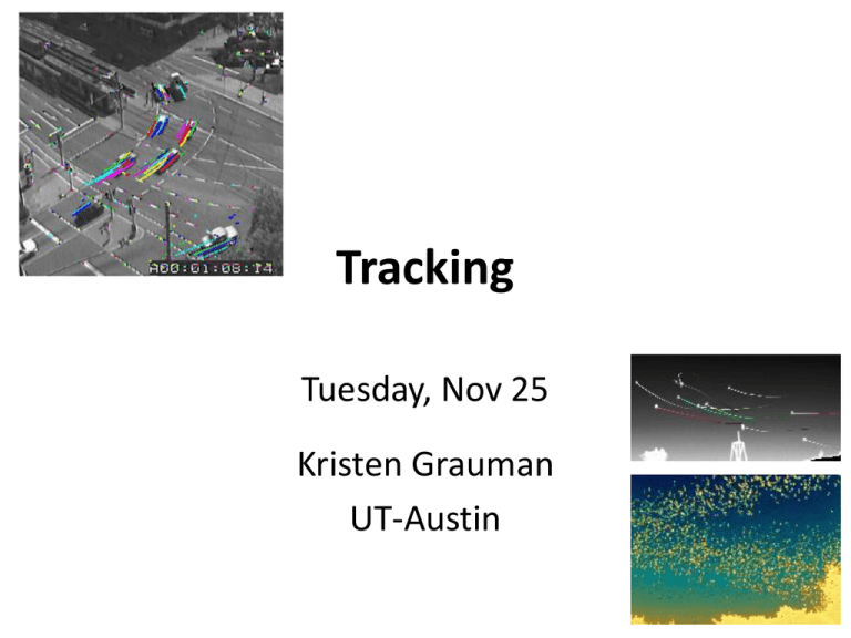
Tracking
Tuesday, Nov 25
Kristen Grauman
UT-Austin
Announcements
• My Wed office hours 1-2 pm
– (and Thurs 2-3 pm)
• Pset 4 out today, due Thurs. Dec 4
– Auto extension to Tues. Dec 9
Pset 4 overview
Part A: 100 pts
Track a corner through the
video with feature-based
matching
Part B: 25 pts
Generalize to multiple tracks,
allow new tracks to form as
new vehicles enter the
frame.
E.C.: bg sub, Kalman filtering
Outline
• Last time: Motion
– Motion field and parallax
– Optical flow, brightness constancy
– Aperture problem
• Today:
– Using optical flow (dense motion estimates) to
recognize activities
– Tracking
• Tracking as inference
• Linear models of dynamics
• Kalman filters
Motion estimation techniques
• Direct methods
• Directly recover image motion at each pixel from spatio-temporal
image brightness variations
• Dense motion fields, but sensitive to appearance variations
• Suitable for video and when image motion is small
Direct methods: Estimating optical flow
I(x,y,t–1)
I(x,y,t)
• Given two subsequent frames, estimate the apparent
motion field between them.
• Key assumptions
• Brightness constancy: projection of the same point looks the
same in every frame
• Small motion: points do not move very far
• Spatial coherence: points move like their neighbors
Solving the aperture problem (grayscale image)
• How to get more equations for a pixel?
• Spatial coherence constraint: pretend the pixel’s
neighbors have the same (u,v)
• If we use a 5x5 window, that gives us 25 equations per pixel
Using optical flow:
recognizing facial expressions
Recognizing Human Facial Expression (1994)
by Yaser Yacoob, Larry S. Davis
Using optical flow:
recognizing facial expressions
Using optical flow:
action recognition at a distance
• Features = optical flow within a region of interest
• Classifier = nearest neighbors
Challenge: low-res
data, not going to
be able to track
each limb.
The 30-Pixel Man
[Efros, Berg, Mori, & Malik 2003]
http://graphics.cs.cmu.edu/people/efros/research/action/
Using optical flow:
action recognition at a distance
Correlation-based tracking
Extract person-centered frame window
[Efros, Berg, Mori, & Malik 2003]
http://graphics.cs.cmu.edu/people/efros/research/action/
Using optical flow:
action recognition at a distance
Extract optical flow to describe the region’s motion.
[Efros, Berg, Mori, & Malik 2003]
http://graphics.cs.cmu.edu/people/efros/research/action/
Using optical flow:
action recognition at a distance
Input
Sequence
Matched
Frames
Use nearest neighbor classifier to name the
actions occurring in new video frames.
[Efros, Berg, Mori, & Malik 2003]
http://graphics.cs.cmu.edu/people/efros/research/action/
Using optical flow:
action recognition at a distance
Input
Sequence
Matched NN
Frame
Use nearest neighbor classifier to name the
actions occurring in new video frames.
[Efros, Berg, Mori, & Malik 2003]
http://graphics.cs.cmu.edu/people/efros/research/action/
Do as I do: motion retargeting
• Include constraint for similarity within sequence as well as
across sequences
Optical flow for tracking?
If we have more than just a pair of frames, we could
compute flow from one to the next:
…
…
But flow only reliable for small motions, and we may have
occlusions, textureless regions that yield bad estimates
anyway…
Motion estimation techniques
• Direct methods
• Directly recover image motion at each pixel from spatio-temporal
image brightness variations
• Dense motion fields, but sensitive to appearance variations
• Suitable for video and when image motion is small
• Feature-based methods
• Extract visual features (corners, textured areas) and track them
over multiple frames
• Sparse motion fields, but more robust tracking
• Suitable when image motion is large (10s of pixels)
Feature-based matching for motion
Interesting point
Best matching
neighborhood
Search
window
Search window is centered at the point
where we last saw the feature, in image I1.
Best match = position where we have the
highest normalized cross-correlation value.
Time t
Time t+1
Feature-based matching for motion
• For a discrete matching search, what are the
tradeoffs of the chosen search window size?
• Which patches to track?
• Select interest points – e.g. corners
• Where should the search window be placed?
• Near match at previous frame
• More generally, according to expected dynamics of the
object
Detection vs. tracking
…
t=1
t=2
t=20
t=21
Detection vs. tracking
…
Detection: We detect the object independently in
each frame and can record its position over time,
e.g., based on blob’s centroid or detection
window coordinates
Detection vs. tracking
…
Tracking with dynamics: We use image
measurements to estimate position of object, but
also incorporate position predicted by dynamics,
i.e., our expectation of object’s motion pattern.
Detection vs. tracking
…
Tracking with dynamics: We use image
measurements to estimate position of object, but
also incorporate position predicted by dynamics,
i.e., our expectation of object’s motion pattern.
Tracking with dynamics
• Use model of expected motion to predict where
objects will occur in next frame, even before seeing
the image.
• Intent:
– Do less work looking for the object, restrict the search.
– Get improved estimates since measurement noise is
tempered by smoothness, dynamics priors.
• Assumption: continuous motion patterns:
– Camera is not moving instantly to new viewpoint
– Objects do not disappear and reappear in different
places in the scene
– Gradual change in pose between camera and scene
Notation reminder
x ~ N (μ, Σ)
• Random variable with Gaussian probability
distribution that has the mean vector μ and
covariance matrix Σ.
• x and μ are d-dimensional, Σ is d x d.
d=2
d=1
If x is 1-d, we
just have one
Σ parameter  the
variance: σ2
Tracking as inference
• The hidden state consists of the true parameters
we care about, denoted X.
• The measurement is our noisy observation that
results from the underlying state, denoted Y.
State vs. observation
Hidden state : parameters of interest
Measurement : what we get to directly observe
Tracking as inference
• The hidden state consists of the true parameters
we care about, denoted X.
• The measurement is our noisy observation that
results from the underlying state, denoted Y.
• At each time step, state changes (from Xt-1 to Xt )
and we get a new observation Yt.
• Our goal: recover most likely state Xt given
– All observations seen so far.
– Knowledge about dynamics of state transitions.
Tracking as inference: intuition
measurement
Belief: prediction
Belief: prediction
Corrected prediction
old belief
Time t
Time t+1
Standard independence assumptions
• Only immediate past state influences
current state
• Measurements at time i only depend on
the current state
Tracking as inference
• Prediction:
– Given the measurements we have seen up to
this point, what state should we predict?
PX t y0 ,, yt 1 
• Correction:
– Now given the current measurement, what
state should we predict?
PX t y0 ,, yt 
Tracking as inference
Recursive process:
• Base case: we have an initial prior P(X0) on the state in
absence of any evidence, which we can correct based
on the first measurement Y0=y0.
• Given corrected estimate for frame t:
1) Predict for frame t+1
2) Correct for frame t+1
Questions
• How to represent the known dynamics that govern the
changes in the states?
• How to represent relationship between state and
measurements, plus our uncertainty in the measurements?
• How to compute each cycle of updates?
Representation: We’ll consider the class of linear
dynamic models, with associated Gaussian pdfs.
Updates: via the Kalman filter.
Linear dynamic model
• Describe the a priori knowledge about
– System dynamics model: represents evolution
of state over time, with noise.
xt ~ N (Dxt 1; Σ d )
nx1
nxn
nx1
– Measurement model: at every time step we
get a noisy measurement of the state.
y t ~ N (Mxt ; Σ m )
mx1
mxn
nx1
Example: randomly
drifting points
xt ~ N (Dxt 1; Σ d )
• Consider a stationary object, with state as position
• Position is constant, only motion due to random
noise term.
• State evolution is described by identity matrix D=I
Example: Constant
velocity (1D points)
1 d position
1 d position
measurements
states
time
Example: Constant
velocity (1D points)
xt ~ N (Dxt 1; Σ d )
y t ~ N (Mxt ; Σ m )
• State vector: position p and velocity v
 pt 
xt   
 vt 
pt  pt 1  (t )vt 1  
vt  vt 1  
1 t   pt 1 
xt  Dt xt 1  noise  
 noise



0 1   vt 1 
• Measurement is position only
 pt 
yt  Mxt  noise  1 0   noise
 vt 
(greek letters
denote noise
terms)
Example: Constant
acceleration (1D points)
Example: Constant
acceleration (1D points)
xt ~ N (Dxt 1; Σ d )
y t ~ N (Mxt ; Σ m )
• State vector: position p, velocity v, and acceleration a.
 pt 
xt   vt 
 at 
pt  pt 1  (t )vt 1  
vt  vt 1  (t )at 1  
at  at 1  
1 t 0   pt 1 
xt  Dt xt 1  noise  0 1 t   vt 1   noise
0 0 1   at 1 
• Measurement is position only
 pt 
yt  Mxt  noise  1 0 0 vt   noise
 at 
(greek letters
denote noise
terms)
Questions
• How to represent the known dynamics that govern the
changes in the states?
• How to represent relationship between state and
measurements, plus our uncertainty in the measurements?
• How to compute each cycle of updates?
Representation: We’ll consider the class of linear
dynamic models, with associated Gaussian pdfs.
Updates: via the Kalman filter.
The Kalman filter
• Method for tracking linear dynamical models in
Gaussian noise
• The predicted/corrected state distributions are
Gaussian
– Only need to maintain the mean and covariance
– The calculations are easy (all the integrals can be
done in closed form)
Kalman filter
Know corrected state
from previous time step,
and all measurements up
to the current one 
Predict distribution over
next state.
Receive
measurement
Time update
(“Predict”)
Measurement update
(“Correct”)
PX t y0 ,, yt 1 
Mean and std. dev.
of predicted state:
 ,

t

t
Know prediction of
state, and next
measurement 
Update distribution over
current state.
PX t y0 ,, yt 
Time advances: t++
Mean and std. dev.
of corrected state:
 ,

t

t
Kalman filter for 1d state
Want to
represent
and update

Px y ,, y   N 

) 
Pxt y0 ,, yt 1   N  , ( )
t
0
t

t

t
 2
t
, (
 2
t
1D Kalman filter: Prediction
• Have linear dynamic model defining predicted state
evolution, with noise

X t ~ N dxt 1 , 
2
d

• Want to estimate predicted distribution for next state

PX t y0 ,, yt 1   N  , ( )

t
• Update the mean:
  d

t

t 1
• Update the variance:
( )    (d )
 2
t
2
d
 2
t 1
 2
t

1D Kalman filter: Correction
• Have linear model defining the mapping of state
to measurements:

Yt ~ N mxt , 
2
m

• Want to estimate corrected distribution given
latest meas.:

 2

PX t y0 ,, yt   N t , ( t )
• Update the mean:

   my ( )
 
2
 m  m ( )

t
• Update the variance:

t
 2
t
t
2
 2
t
2
m
 ( )
( )  2
 m  m ( )
 2
t
2
m
 2
t
2
 2
t
Prediction vs. correction
   my ( )
 
2
 m  m ( )

t

t
 2
t
t
2
 2
t
2
m
 ( )
( )  2
 m  m ( )
 2
t
2
m
 2
t
2
 2
t
• What if there is no prediction uncertainty ( t  0) ?
 

t

t
( )  0
 2
t
The measurement is ignored!
• What if there is no measurement uncertainty ( m  0) ?
yt
 
m

t
( )  0
 2
t
The prediction is ignored!
Recall: constant velocity example
position
measurements
state
time
State is 2d: position + velocity
Measurement is 1d: position
Constant velocity model
Kalman filter processing
o state
x measurement
* predicted mean estimate
position
+ corrected mean estimate
bars: variance estimates
before and after measurements
time
Constant velocity model
Kalman filter processing
o state
x measurement
* predicted mean estimate
position
+ corrected mean estimate
bars: variance estimates
before and after measurements
time
Constant velocity model
Kalman filter processing
o state
x measurement
* predicted mean estimate
position
+ corrected mean estimate
bars: variance estimates
before and after measurements
time
Constant velocity model
Kalman filter processing
o state
x measurement
* predicted mean estimate
position
+ corrected mean estimate
bars: variance estimates
before and after measurements
time
Kalman filter: General case (> 1dim)
What if state vectors have more than one dimension?
PREDICT
CORRECT
xt  Dt xt1

t

t 1
  Dt  D  dt
T
t

t


 K y  M x 

t
Kt   M M t  M  mt
xt  xt
T
t
t
t
 t  I  K t M t  t
T
t
1

t t
More weight on residual
when measurement error
covariance approaches 0.
Less weight on residual as a
priori estimate error
covariance approaches 0.
Tracking: issues
• Initialization
– Often done manually
– Background subtraction, detection can also be used
• Data association, multiple tracked objects
– Occlusions
Data association
• We’ve assumed entire
measurement (y) was cue
of interest for the state
• But, there are typically
uninformative
measurements too–clutter.
• Data association: task of
determining which
measurements go with
which tracks.
Data association
• Simple strategy: only pay attention to the
measurement that is “closest” to the
prediction
Source: Lana Lazebnik
Data association
• Simple strategy: only pay attention to the
measurement that is “closest” to the
prediction
Doesn’t always work…
Alternative: keep track of multiple hypotheses at once…
Source: Lana Lazebnik
• http://www.cs.bu.edu/~betke/research/bats/
Tracking: issues
• Initialization
– Often done manually
– Background subtraction, detection can also be used
• Data association, multiple tracked objects
– Occlusions
• Deformable and articulated objects
• Constructing accurate models of dynamics
– E.g., Fitting parameters for a linear dynamics model
• Drift
– Accumulation of errors over time
Drift
D. Ramanan, D. Forsyth, and A. Zisserman. Tracking People by Learning their
Appearance. PAMI 2007.
Source: Lana Lazebnik
Summary
• Using optical flow to recognize activities
– Low-level feature captures motion patterns in a region
of interest
• Tracking as inference
– Goal: estimate posterior of object position given
measurement
• Linear models of dynamics
– Represent state evolution and measurement models
• Kalman filters
– Recursive prediction/correction updates to refine
measurement