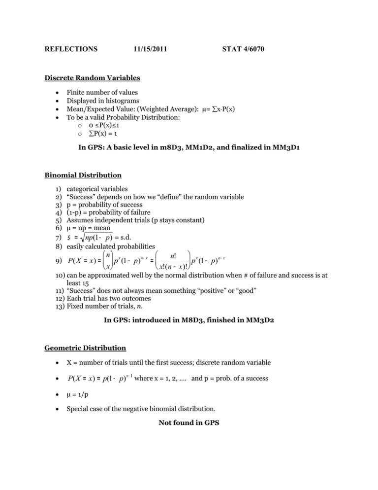
REFLECTIONS
11/15/2011
STAT 4/6070
Discrete Random Variables




Finite number of values
Displayed in histograms
Mean/Expected Value: (Weighted Average): µ= xP(x)
To be a valid Probability Distribution:
o 0 ≤P(x)≤1
o P(x) = 1
In GPS: A basic level in m8D3, MM1D2, and finalized in MM3D1
Binomial Distribution
1)
2)
3)
4)
5)
6)
7)
8)
categorical variables
“Success” depends on how we “define” the random variable
p = probability of success
(1-p) = probability of failure
Assumes independent trials (p stays constant)
µ = np = mean
s = np(1- p) = s.d.
easily calculated probabilities
æ nö
æ
n! ö x
n-x
÷ p (1- p)
è x!(n - x)!ø
9) P( X = x) = ç ÷ p x (1- p) n-x = ç
è xø
10) can be approximated well by the normal distribution when # of failure and success is at
least 15
11) “Success” does not always mean something “positive” or “good”
12) Each trial has two outcomes
13) Fixed number of trials, n.
In GPS: introduced in M8D3, finished in MM3D2
Geometric Distribution

X = number of trials until the first success; discrete random variable

P(X = x) = p(1- p)x-1 where x = 1, 2, …. and p = prob. of a success

µ = 1/p

Special case of the negative binomial distribution.
Not found in GPS
Normal Distribution (Continuous R. Variable)




z-score probability
Probability distribution  symmetric, bell-shaped graph
Mean and Standard deviation parameters
Empirical Rule (Image from our textbook, p. 280)



Standard Normal Distribution  µ=0, =1
Cumulative Probability: (Image from textbook, p 282.)


Continuous random variable has possible values that form an interval
Probability is between 0 and 1.
In GPS: MM3D2 taught along with Binomial.
Adding/Subtracting Two Independent Random Variables

The sum of the means = mean of total mx ± y = mx ± m y

The square root of the sums of the squares of the standard deviations (of the parts) is the
standard deviation of the total (or difference)
s 2x + y = s 2x + s 2y
s 2x- y = s 2x + s 2y
In GPS: a slight link to MM1D2
Frequentist versus Bayesian Probability
FREQUENTIST
BAYESIAN
Long run relative frequency
 is fixed and unknown
 never gets assigned probability
Probability is evidence based – degree belief
 must be given a distribution
 has probability but no agreement on dist.
I didn’t find this topic in GPS
Confidence Interval for a Proportion
Estimate  margin of error  sample proportion  z (standard error of sample proportion)
Contains a range of plausible values for the population proportion at a specified confidence level
If using 95% confidence level, in repeated sampling, if we build an interval using the above
procedure, we expect 95% of the intervals to capture the population proportion.
In GPS: MM4d2 and MM4d3