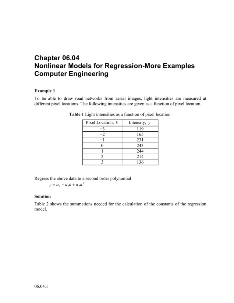
Chapter 06.04
Nonlinear Models for Regression-More Examples
Computer Engineering
Example 1
To be able to draw road networks from aerial images, light intensities are measured at
different pixel locations. The following intensities are given as a function of pixel location.
Table 1 Light intensities as a function of pixel location.
Pixel Location, k
−3
−2
−1
0
1
2
3
Intensity, y
119
165
231
243
244
214
136
Regress the above data to a second order polynomial
y  a0  a1 k  a 2 k 2
Solution
Table 2 shows the summations needed for the calculation of the constants of the regression
model.
06.04.1
06.04.2
Chapter 06.04
Table 2 Summations for calculating constants of model.
i
1
2
3
4
5
6
7
Pixel Location, k
Intensity, y
k2
k3
k4
ky
k2  y
−3
−2
−1
0
1
2
3
119
165
231
243
244
214
136
9
4
1
0
1
4
9
−27
−8
−1
0
1
8
27
81
16
1
0
1
16
81
−357
−330
−231
0
244
428
408
1071
660
231
0
244
856
1224
0
1352
28
0
196
162
4286
7

i 1
y  a 0  a1 k  a 2 k 2 is the quadratic relationship between the pixel location and intensity
where the coefficients a 0 , a1 , a 2 are found as follows

 n


 n
  k i 
 i n1 
 k 2 
i
 
 i 1 
 n

  ki 
 i 1 
 n 2
  ki 
 i 1 
 n 3
  ki 
 i 1 
n7
7
k
i 1
i
7
k
i 1
2
i
28
3
i
0
4
i
 196
7
k
i 1
7
k
i 1
7
y
i 1
0
i
 1352
7
k y
i 1
i
7
k
i 1
2
i
i
162
y i  4286
 n 2 
 n
  ki  
 yi
 i 1   a   i 1
0
 n 3     n
  k i   a1    k i yi
 i 1      i 1
a
n
 n 4   2   k 2 y
  ki  
 i i
 i 1
 i 1  








Nonlinear Models for Regression-More Examples: Computer Engineering
06.04.3
We have
 7 0 28  a 0  1352 
 0 28 0   a    162 

 1  

28 0 196 a 2  4286
Solve the above system of simultaneous linear equations, we get
a 0   246.57 
 a    5.7857 
 1 

a 2   13.357
The polynomial regression model is
P  a 0  a1 m  a 2 m 2
 246.57  5.7857m  13.357m 2
Figure 1 Second order polynomial regression model for intensity as a function of pixel
location.