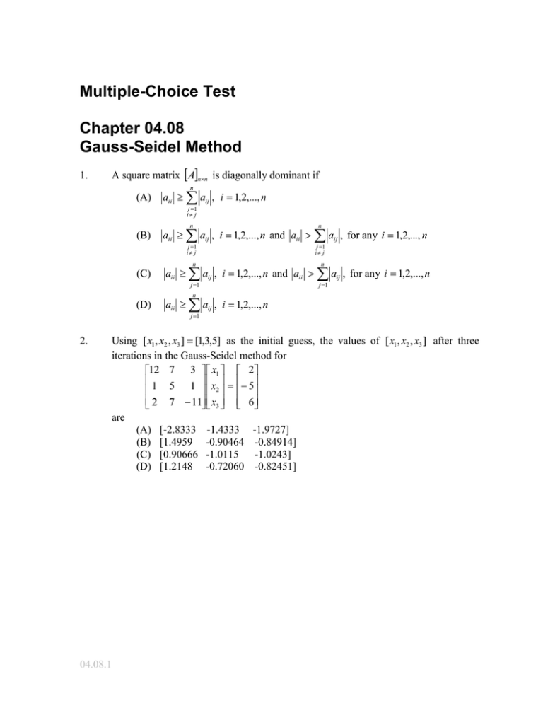
Multiple-Choice Test
Chapter 04.08
Gauss-Seidel Method
1.
A square matrix Ann is diagonally dominant if
n
(A)
aii   aij , i  1,2,..., n
j 1
i j
(B)
(C)
n
n
j 1
i j
j 1
i j
n
n
j 1
j 1
aii   aij , i  1,2,..., n and aii   aij , for any i  1,2,..., n
aii   aij , i  1,2,..., n and aii   aij , for any i  1,2,..., n
n
(D)
aii   aij , i  1,2,..., n
j 1
2.
Using [ x1 , x2 , x3 ]  [1,3,5] as the initial guess, the values of [ x1 , x2 , x3 ] after three
iterations in the Gauss-Seidel method for
12 7 3   x1   2
 1 5 1   x    5

 2   
 2 7  11  x3   6
are
(A)
(B)
(C)
(D)
04.08.1
[-2.8333
[1.4959
[0.90666
[1.2148
-1.4333
-0.90464
-1.0115
-0.72060
-1.9727]
-0.84914]
-1.0243]
-0.82451]
04.08.2
3.
Chapter 04.08
To ensure that the following system of equations,
2 x1  7 x2  11x3 
6
x1  2 x2 
x3   5
7 x1  5 x2  2 x3  17
converges using the Gauss-Seidel method, one can rewrite the above equations as
follows:
2 7  11  x1   6 
(A) 1 2 1   x2    5

   
7 5 2   x3   17 
(B)
7 5 2   x1   17 
1 2 1   x    5

  2  
2 7  11  x3   6 
7 5 2   x1   6 
(C) 1 2 1   x2    5
2 7  11  x3   17 
(D) The equations cannot be rewritten in a form to ensure convergence.
4.
12 7 3   x1   22 
For  1 5 1   x2    7  and using x1
 2 7  11  x3   2
the values of x1
Iteration #
1
2
3
4
x2
x2
x3   1 2 1 as the initial guess,
x3  are found at the end of each iteration as
x1
0.41667
0.93990
0.98908
0.99899
x2
1.1167
1.0184
1.0020
1.0003
x3
0.96818
1.0008
0.99931
1.0000
At what first iteration number would you trust at least 1 significant digit in your
solution?
(A) 1
(B) 2
(C) 3
(D) 4
04.08.2
04.08.3
5.
Chapter 04.08
The algorithm for the Gauss-Seidel method to solve AX   C  is given as follows
when using n max iterations. The initial value of X  is stored in X  .
(A) Sub Seidel (n, a, x, rhs, nmax )
For k  1 To nmax
For i  1 To n
For j  1 To n
If ( i  j ) Then
Sum = Sum + a (i, j ) * x( j )
endif
Next j
x(i )  (rhs (i )  Sum) / a(i, i )
Next i
Next j
End Sub
(B) Sub Seidel (n, a, x, rhs, nmax)
For k  1 To nmax
For i  1 To n
Sum = 0
For j  1 To n
If ( i  j ) Then
Sum = Sum + a (i, j ) * x( j )
endif
Next j
x(i )  (rhs (i )  Sum) / a(i, i )
Next i
Next k
End Sub
(C) Sub Seidel (n, a, x, rhs, nmax)
For k  1 To nmax
For i  1 To n
Sum = 0
For j  1 To n
Sum = Sum + a (i, j ) * x( j )
Next j
x(i )  (rhs (i )  Sum) / a(i, i )
Next i
04.08.4
Chapter 04.08
Next k
End Sub
(D) Sub Seidel (n, a, x, rhs, nmax )
For k  1 To nmax
For i  1 To n
Sum = 0
For j  1 To n
If ( i  j ) Then
Sum = Sum + a (i, j ) * x( j )
endif
Next j
x(i )  (rhs (i )  Sum) / a(i, i )
Next i
Next k
End Sub
6.
Thermistors measure temperature, have a nonlinear output and are valued for a
limited range. So when a thermistor is manufactured, the manufacturer supplies a
resistance vs. temperature curve. An accurate representation of the curve is generally
given by
1
2
3
 a 0  a1 ln( R)  a 2 ln R   a3 ln R 
T
where T is temperature in Kelvin, R is resistance in ohms, and a0 , a1 , a2 , a3 are
constants of the calibration curve. Given the following for a thermistor
R
T
ohm
C
1101.0 25.113
911.3 30.131
636.0 40.120
451.1 50.128
the value of temperature in C for a measured resistance of 900 ohms most nearly is
(A) 30.002
(B) 30.473
(C) 31.272
(D) 31.445
For a complete solution, refer to the links at the end of the book.
04.08.2