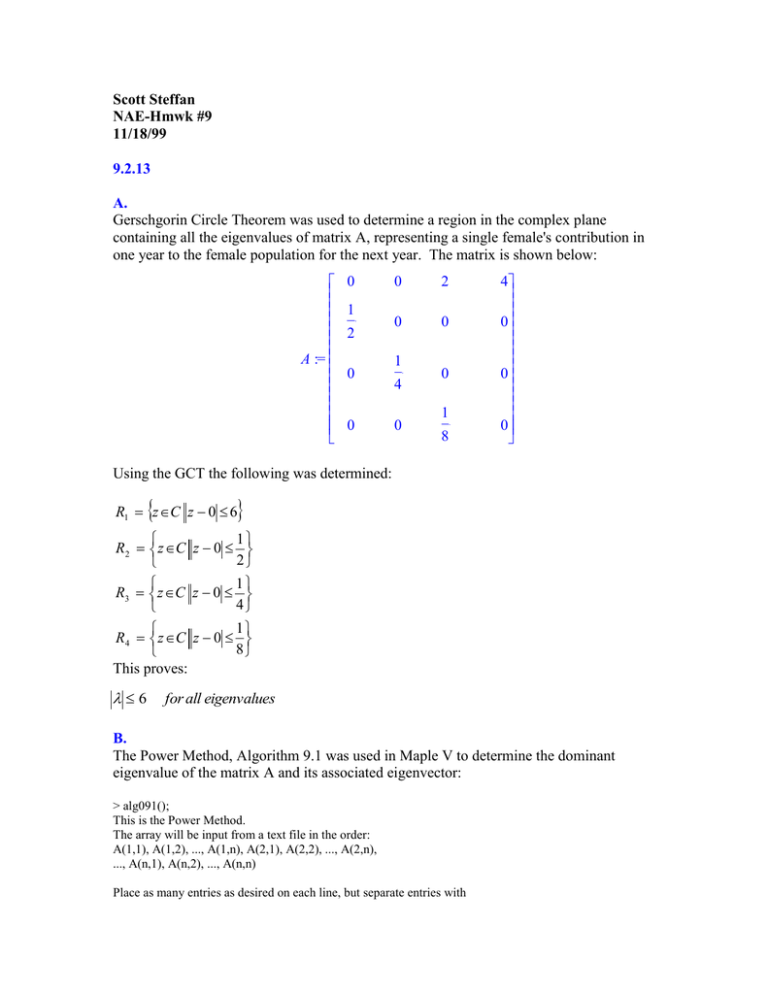
Scott Steffan
NAE-Hmwk #9
11/18/99
9.2.13
A.
Gerschgorin Circle Theorem was used to determine a region in the complex plane
containing all the eigenvalues of matrix A, representing a single female's contribution in
one year to the female population for the next year. The matrix is shown below:








A := 








0
1
2
0
0
0
2
0
0
1
4
0
0
1
8
4



0




0




0

Using the GCT the following was determined:


R1  z C z  0  6
1

R 2   z C z  0  
2

1

R3   z C z  0  
4

1

R 4   z C z  0  
8

This proves:
6
for all eigenvalues
B.
The Power Method, Algorithm 9.1 was used in Maple V to determine the dominant
eigenvalue of the matrix A and its associated eigenvector:
> alg091();
This is the Power Method.
The array will be input from a text file in the order:
A(1,1), A(1,2), ..., A(1,n), A(2,1), A(2,2), ..., A(2,n),
..., A(n,1), A(n,2), ..., A(n,n)
Place as many entries as desired on each line, but separate entries with
at least one blank.
The initial approximation should follow in same format.
Input the file name in the form - drive:\name.ext
for example: A:\DATA.DTA
> C:\Numerical_Analysis\Hmwk9\9213b.dta
Input the dimension n.
>4
Input the tolerance.
> 0.00000001
Input maximum number of iterations - integer.
> 150
Choice of output method:
1. Output to screen
2. Output to text file
Please enter 1 or 2.
>1
POWER METHOD
The solution took 143 iterations to generate a solution of the specified tolerance above.
The following spreadsheet summarizes the beginning and ending iterations:
Iteration Approx Eigenvalue Eigenvector
1
2
1
0.25000000 0.12500000 0.06250000
2
0.5
1
1.00000000 0.12500000 0.03125000
3
0.375
0.75
1.00000000 0.50000000 0.03125000
4
0.375
1
0.33333333 0.22222222 0.05555556
5
0.66666667
1
0.75000000 0.12500000 0.04166667
139
0.69766851
1
0.71667273 0.25680991 0.04601217
140
0.6976685
1
0.71667275 0.25680991 0.04601217
141
0.69766849
1
0.71667276 0.25680992 0.04601217
142
0.69766851
1
0.71667274 0.25680992 0.04601217
143
0.6976685
1
0.71667275 0.25680991 0.04601217
The eigenvalue := .69766850 to tolerance := 1.0000000000e-08
obtained on iteration number := 143
Unit eigenvector is :
1.00000000 .71667275 .25680991 .04601217
C.
Wielandt Deflation, Algorithm 9.4 was to be used to determine the remaining eigenvalues
and eigenvectors of A once the dominants are known. The vector x was calculated as
shown below:
1
ai1 , ai 2, ... ain t
(1)
1vi
The Wielandt code does not have the capability to handle complex eigenvalues so no
converged solution was generated using this method. For this reason, Muller's Method,

x
Algorithm 2.8 was used in Maple V to generate the complex eigenvalues, with the
characteristic polynomial determined in part D of this problem. The following shows
the 2nd and 3rd, and 4th eigenvalues:
> alg028();
This is Muller's Method.
Input the Polynomial P(x) in terms of x
> x^4-x/4-1/16
For example: x^2-2*x+2Input tolerance
> .00001
Input maximum number of iterations - no decimal point
> 30
Input the first of three starting values
> -1 -2 -3
Input the second of three starting values
Input the third starting value
Select output destination
1. Screen
2. Text file
Enter 1 or 2
>1
MULLER'S METHOD
The output is i, approximation x(i), f(x(i))
Three columns means the results are real numbers,
Five columns means the results are complex
numbers with real and imaginary parts of x(i)
followed by real and imaginary parts of f(x(i)).
3 -1.195000000+.9733961166e-1*I 2.194411955-.6843625902*I
4 -1.209358052+.3269935575*I 1.452020762-2.226083871*I
5 -.9772536486+.4458263222*I -.553905020e-2-1.429428590*I
6 -.6711460726+.5097020094*I -.3264567498-.3882867085*I
7 -.4982237502+.5552874326*I -.2404872207-.7229435783e-1*I
8 -.3529326402+.5708432599*I -.9610430145e-1+.195126665e-1*I
9 -.2634132630+.5745461836*I -.2029236758e-1+.141941752e-1*I
10 -.2332783240+.5714259365*I -.121413672e-2+.22333395e-2*I
11 -.2301950473+.5697078557*I .806327e-5+.358804e-4*I
12 -.2301775766+.5696588531*I .1542e-7+.11e-8*I

(13)
-.2301775942+.5696588401*I = 2
Various trial and error x0, x1, and x2 values within the Gerschgorin Circle bounds to
determine all of the eigenvalues:



(13)
(9)
(6)
-.2301775942 - .5696588401*I = 3
-.2373133088 = 4
.6976684973 = 1
D.
The real eigenvalues of A were determined by using the Newton-Raphson Method,
Algorithm 2.3 in Maple V. This requires the determination of a characteristic polynomial
to represent the matrix A. Using the following, the characteristic polynomial of A is
created:
P(  )  det ( A  I )
1
4 1
P(  ) :=   
4
16
The results are shown below:
> alg023();
This is Newton's Method
Input the function F(x) in terms of x
> x^4-x/4-1/16
For example: cos(x)Input initial approximation
>6
Input tolerance
> .00000001
Input maximum number of iterations - no decimal point
> 50
Select output destination
1. Screen
2. Text file
Enter 1 or 2
>1
Select amount of output
1. Answer only
2. All intermeditate approximations
Enter 1 or 2
>2
 Approximate solution = 6.9766849720e-01
with F(P) = 0.0000000000e-01
 Number of iterations = 13
Tolerance = 1.0000000000e-08
= 1
Using an approximate solution of -6, the other bound, the following is generated:
 Approximate solution = -2.3731330880e-01
with F(P) = 1.0000000000e-11
 Number of iterations = 14
Tolerance = 1.0000000000e-08
= 4
E.
Since matrix A converges, I would predict the beetle would eventually become extinct.
Their population will approach zero.