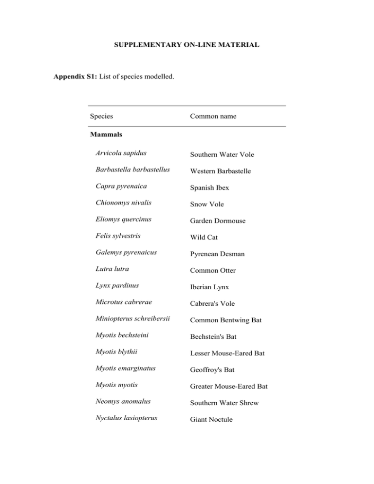
SUPPLEMENTARY ON-LINE MATERIAL
Appendix S1: List of species modelled.
Species
Common name
Mammals
Arvicola sapidus
Southern Water Vole
Barbastella barbastellus
Western Barbastelle
Capra pyrenaica
Spanish Ibex
Chionomys nivalis
Snow Vole
Eliomys quercinus
Garden Dormouse
Felis sylvestris
Wild Cat
Galemys pyrenaicus
Pyrenean Desman
Lutra lutra
Common Otter
Lynx pardinus
Iberian Lynx
Microtus cabrerae
Cabrera's Vole
Miniopterus schreibersii
Common Bentwing Bat
Myotis bechsteini
Bechstein's Bat
Myotis blythii
Lesser Mouse-Eared Bat
Myotis emarginatus
Geoffroy's Bat
Myotis myotis
Greater Mouse-Eared Bat
Neomys anomalus
Southern Water Shrew
Nyctalus lasiopterus
Giant Noctule
Nyctalus leisleri
Lesser Noctule
Plecotus auritus
Brown long-eared Bat
Plecotus austriacus
Grey long-eared Bat
Rhinolophus euryale
Mediterranean Horseshoe Bat
Rhinolophus ferrumequinum
Greater Horseshoe Bat
Rhinolophus hipposideros
Lesser Horseshoe Bat
Rhinolophus mehelyi
Mehely's Horseshoe Bat
Sciurus vulgaris
Red Squirrel
Birds
Actitis hypoleucos
Common Sandpiper
Aegypius monachus
Cinereus Vulture
Alcedo atthis
Common Kingfisher
Anas strepera
Gadwall
Apus pallidus
Pallid Swift
Aquila adalberti
Spanish Imperial Eagle
Aquila chrysaetus
Golden Eagle
Ardea purpurea
Purple Heron
Asio flammeus
Short-eared Owl
Bubo bubo
Eurasian Eagle-Owl
Burhinus oedicnemus
Eurasian Thick-Knee
Caprimulgus ruficollis
Red-necked nightjars
Ciconia ciconia
Storks White Stork
Ciconia nigra
Black Stork
Cinclus cinclus
White-Throated Dipper
Circus aeruginosus
Western Marsh Harrier
Circaetus gallicus
Short-Toed Snake-Eagle
Circus pygargus
Montagu’s Harrier
Coracias garrulous
Eurasian Roller
Dendrocopos minor
Lesser Spotted Woodpecker
Egretta garzetta
Little Egret
Elanus caeruleus
Black-winged Kite
Emberiza schoeniclus
Reed Bunting
Falco naumanni
Lesser Kestrel
Falco peregrinus
Peregrine Falcon
Falco subbuteo
Eurasian Hobby
Gyps fulvus
Eurasian Griffon
Hieraaetus fasciatus
Bonelli's Eagle
Hieraaetus pennatus
Booted Eagle
Himantopus himantopus
Black-winged Stilt
Ixobrychus minutus
Little Bittern
Jynx torquilla
Wryneck
Lanius excubitor
Great Grey Shrike
Luscinia svecica
Bluethroat
Melanocorypha calandra
Calandra Lark
Milvus milvus
Red Kite
Netta rufina
Red-crested Pochard
Nycticorax nycticorax
Black-crowned night-heron
Oenanthe leucura
Black Wheater
Otis tarda
Great Bustard
Panurus biarmicus
Bearded Parrotbill
Pernis apivorus
Honey Buzzard
Phoenicurus phoenicurus
Common Redstart
Podiceps nigricollis
Black-necked Grebe
Prunella collaris
Alpine Accentor
Pterocles alchata
Pin-Tailed Sandgrouse
Pterocles orientales
Black-bellied Sandgrouse
Pyrrhocorax pyrrhocorax
Red-Billed Chough
Rallus aquaticus
Water Rail
Riparia riparia
Sand Martin
Saxicola rubetra
Whinchat
Serinus citrinella
Citril Finch
Sylvia hortensis
Orphean Warbler
Tetrax tetrax
Little Bustard
Tyto alba
Barn owl
Vanellus vanellus
Lapwing
Herptiles
Hyla arborea
Common Tree Frog
Rana iberica
Iberian Frog
Pelodytes punctatus
Parsley Frog
Alytes cisternasii
Iberian Midwife Toad
Lissotriton boscai
Bosca's newts
Triturus pygmaeus
Southern Marbled Newt
Mesotriton alpestris
Alpine Newt
Hemorrhois hippocrepis
Horseshoe Whip Snake
Macroprotodon cucullatus
False Smoth Snake
Mauremys leprosa
Spanish turtle
Emys orbicularis
European Pond Turtle
Lacerta monticola
Iberian Rock Lizard
Lacerta schreiberi
Schreiber's Green Lizard
Appendix S2: Generation of pseudo-absences
Species distributions are not only constrained by abiotic factors (e.g. climate), but also
by biotic interactions, dispersal constrains, anthropogenic effects, stochastic events and
other historical, unique and contingent events that may preclude the presence of a given
species in a priori environmentally suitable places. Thus, if the goal is to predict
environmentally suitable areas (i.e. potential distributions regarding environmental
suitability), only absences due to unsuitable environmental conditions (i.e.
environmental pseudo-absences) should be used to build predictive models (Peterson,
Papes & Soberón, 2008; Jiménez-Valverde, Lobo & Hortal, 2008). Here, pseudoabsences were obtained using multi-dimensional niche envelopes over all peninsular
Spain (Lobo, Verdú & Numa, 2006 and references therein), in which presence data were
used to calculate an environmental range for each species. Pseudo-absences correspond
to the observed absences that lay outside each species’ environmental range (i.e. outside
the maximum and minimum for the variables considered). Lastly, both presences and
pseudo-absences were included as a binomial dependent variable in GLMs, in order to
estimate the potential species’ distributions. GLMs including pseudo-absences
generated by the multi-dimensional niche envelope model give predictions closer to the
potential species’ distributions (Chefaoui and Lobo, 2008). Assuming that there is not a
strong methodological bias in the presence data, as in the present study, this procedure
enables to reduce the effect of factors, such as dispersal constraints, that preclude the
characterization of the entire species’ potential distribution.
Appendix S3: Does the use of pseudo-absences increase inter-model consistency
regarding potential distributions?
This investigation pursues generating models able to predict species’ potential
distributions (i.e. environmentally suitable areas) through space and time, for which we
combined observed presences and pseudo-absences under the expectation that pseudoabsences would reduce prediction errors (Chefaoui and Lobo, 2008). To investigate this,
we took into account that predictions often vary among different modelling techniques
(e.g. Araújo et al., 2005), and assumed that the most robust results should be those that
are less dependent on the technique used for modelling. Specifically, we compared the
results provided by our General Linear Models (GLMs) when using all observed
absences or only pseudo-absences, with the results generated by other two widely
employed modelling techniques: Neural Networks (NNTs) and Classification Tree
Analyses (TREEs). That is, for each species and technique we obtained two sets of
probabilities over all peninsular Spain (modelling either with all absences or only with
pseudo-absences), and then examined to what extent the degree of agreement of GLMs
with the other models was dependent on the type of data used. Thus, for each species
we performed Pearson’s correlations between the obtained probabilities using GLMs
and those obtained using the alternative technique (either NNTs or TREEs) for both
types of data separately. We compared between the two types of data used, the
correlation coefficients obtained for each species. We found that the use of pseudoabsences increased inter-model consistency for the set of species modeled (repeated
measures ANOVA; GLM vs. NNT: F1,93 = 42.72, P < 0. 000001; GLM vs. TREE: F1,93
= 104.38, P < 0. 000001; Fig. B). This indeed supports that pseudo-absences give more
robust results in this case.
Correlation coefficients between two modelization techniques for
each species
0.82
0.80
0.78
GLM vs. NNT
GLM vs. TREE
0.76
0.74
0.72
0.70
0.68
0.66
0.64
0.62
0.60
0.58
0.56
0.54
All absences
Only pseudo-absences
Fig. S3 - Pearson correlation coefficients ( X ±SE) between the probabilities obtained
using Generalized Linear Models and Neural Networks (GLM vs. NNT: □) or
Classification Trees (GLM vs. TREE: ◊), for each species modelled for all of peninsular
Spain.
Appendix
S4:
Threshold
to
transform
continuous
probabilities
into
presence/absence data
Logistic models generate continuous probabilities of species presences, and a specific
threshold is needed to transform the probability data to presence/absence data. Among
the different approaches to determine such threshold, we used the prevalence
(presence/absence ratio used for modelling), a method that has already been shown to be
effective for plants (Liu et al., 2005), aquatic invertebrate families (Manel, Williams &
Ormerod, 2001), and simulated species (Jiménez-Valverde and Lobo, 2006).
Additionally, we also followed Jiménez-Valverde and Lobo (2006; 2007) to check
whether this approach worked well for the case of threatened terrestrial vertebrates
analyzed here. We first conducted a jack-knifing resampling technique (Vaughan and
Ormerod, 2005; Pearson et al., 2007) to estimate the fractions of correctly predicted
presences (sensitivity) and correctly predicted absences (specificity) by our GLM
models. The resampling is executed in an iterative way. That is, we excluded one
observation at each time and rebuilt the model with the remaining data to predict the
response of the excluded observation. Then we re-entered this observation into the
dataset and repeated the operation until all observations were predicted. Sensitivity and
specificity were computed for each model based on these predictions, and these were
used to establish the cut-off level that minimizes model prediction error (i.e. the
threshold probability value that minimizes the sensitivity-specificity difference). The
correlation between these cut-off level values and species' prevalences was nearly one
(Pearson’s correlation: R = 0.960, F1,92 = 1086.09, P < 0.000001; Fig. C), thus
supporting prevalence as an appropriate reference to transform model probabilities into
predicted presence/absence data.
Cut-off minimizing sensitivity-specificity difference
1.0
0.8
0.6
0.4
0.2
0.0
0.0
0.2
0.4
0.6
0.8
1.0
Prevalence
Fig. S4 - Relationship between the cut-off that minimized the prediction error
(measured as the minimized sensitivity-specificity difference) and prevalence.
Appendix S5: Evaluation of models
Often, threatened species exhibit low numbers of presences, including some of the
species considered in this study, thus preventing to split the data into training and
validation datasets. Alternatively, model stability can be estimated by comparing
sensitivity and specificity values obtained from direct model predictions with those
provided by the jack-knifing resampling technique described above (Vaughan and
Ormerod, 2005; Pearson et al., 2007). We also calculated for each model the area under
the curve (AUC) of the Receiver Operating Characteristic (ROC) plot of sensitivity
against 1-specificity (Fielding and Bell, 1997), in order to use this estimate as an
additional index of the overall stability of the models. Specifically, we used simple
regressions to perform paired comparisons of the species' values obtained before and
after jack-knifing for sensitivity, specificity and AUC. All relationships were strong,
positive and highly significant (sensitivity: R = 0.945, F1,92 = 766.47, P < 0. 000001;
specificity: R = 0.890, F1,92 = 350.22, P < 0. 000001; AUC: R = 0.751, F1,92 = 118.78, P
< 0.000001), thus denoting small overall bias.
Additionally, to examine whether there were differences in terms of model
stability among animal groups, we took the residuals from the former regressions as
measurements of model stability for each species relative to the other species, and then
compared them among animal groups using one-way ANOVAs. We only compared the
residuals of sensitivity and specificity, since the AUC approach is not recommended to
perform among-species accuracy estimations (Lobo, Jiménez-Valverde & Real, 2007).
Residuals of sensitivity and specificity did not differ significantly among animal groups
(sensitivity: F2,91 = 0.53, P = 0.58; specificity: F2,91= 0.88, P = 0.41), for which we
concluded that there were no biases toward any particular taxa.
Appendix S6: Spatial autocorrelation
It has been shown that the parameter estimation of models is not seriously affected by
the spatial autocorrelation in the residuals of models (Hawkins et al., 2007; Diniz-Filho
et al., 2007). However, since the aim of our study is to examine differences among
animal groups, it is worthwhile to test whether spatial autocorrelation in the residuals of
models differs among them. For this purpose we generated spatial correlograms of
Moran’s I using the spatial analysis in macroecology (SAM) software (Rangel, DinizFilho & Bini, 2006). Specifically, we identified for each species the maximum distances
at which positive spatial autocorrelation remained statistically significant in the data.
We then compared among animal groups and found no significant differences (one-way
ANOVA: F2,91 = 0.48, P = 0.62).
Appendix S7: Range size effect on the proportion of deviance explained by models
It has been shown that the fit or performance of models can be associated with species
occupancy (Manel et al., 2001; Segurado and Araújo, 2004; Schwartz et al., 2006),
therefore we examined this possibility using a Pearson correlation between deviance
explained and species occupancy (number of presences). In fact, even the adjusted
deviance, weighted by the effective degrees of freedom used to fit the model (Guisan et
al., 1999; Engler et al., 2004), significantly correlated with species occupancy
(Pearson’s correlation: R = 0.32, F1,92 = 10.67, P < 0.01). Then, we took the residuals of
this regression as a measurement of range-corrected deviance to verify that the observed
patterns of deviances through functional groups were still the highest for herptiles (oneway ANOVA: F1,91 = 4.52, P = 0.03).
Appendix S8:
Table S8 - Within-group percentage of species for which a given predictor was retained
in the final models after the backward selection procedure (see Methods section). T,
mean annual temperature; mPET, minimum potential evapotranspiration; P, annual
precipitation; tpAET, Turc-Pike’s actual evapotranspiration; WD, water deficit.
Animal Groups
Predictors included in models
% Mammals
% Birds
% Herptiles
T
68
73.2
76.9
mPET
64
76.7
53.8
T+mPET
80
96.4
100
80
55.3
84.6
tpAET
72
55.3
76.9
WD
92
73.2
69.2
tpAET+WD
96
91
100
Acidic deposits
52
35.7
46.1
Basic deposits
44
46.4
23.1
Acidic rocks
48
44.6
53.8
Basic rocks
44
37.5
46.1
Average elevation
48
51.7
53.8
Range of elevation
40
69.6
53.8
Temperature-related predictors
Water-related predictors
P
Temperature- and water-related
predictors
Soil predictors
Topographical predictors
Additional references:
Araújo, M.B., Pearson, R.G., Thuiller, W. & Erhard, M. (2005). Validation of speciesclimate impact models under climate change. Glob. Change Biol. 11, 1504-1513.
Chefaoui, R.M. & Lobo, J.M. (2008). Assessing the effects of pseudo-absences on
predictive distribution model performance. Ecol. Model. 210, 478-486.
Diniz-Filho, J.A.F., Hawkins, B.A., Bini, L.M., De Marco, P. & Blackburn, T.M.
(2007). Are spatial regression methods a panacea or a Pandora’s box? A reply to
Beale et al. (2007). Ecography 30, 848-851.
Fielding, A.H. & Bell, J.F. (1997). A review of methods for the assessment of
prediction errors in conservation presence/ absence models. Environ. Conserv.
24, 38-49.
Hawkins, B.A., Diniz-Filho, J.A.F., Bini, L.M., De Marco, P. & Blackburn, T.M.
(2007). Red herrings revisited: spatial autocorrelation and parameter estimation
in geographical ecology. Ecography 30, 375-384.
Jiménez-Valverde, A., Lobo, J.M. & Hortal, J. (2008). Not as good as they seem: the
importance of concepts in species distribution modelling. Divers. Distrib. 24,
885-890.
Lobo, J.M., Verdú, J.R. & Numa, C. (2006). Environmental and geographical factors
affecting the Iberian distribution of flightless Jekelius species (Coleoptera:
Geotrupidae). Divers. Distrib. 12, 179-188.
Lobo, J.M., Jiménez-Valverde, A. & Real, R. (2007). AUC: a misleading measure of
the performance of predictive distribution models. Global Ecol. Biogeogr. 17,
145–151.
Manel, S., Williams, H.C. & Ormerod, S.J. (2001). Evaluating presence-absence models
in ecology: the need to account for prevalence. J. Appl. Ecol. 38, 921-931.
Peterson, A.T., Papes, M. & Soberón, J. (2008). Rethinking receiver operating
characteristic analysis applications in ecological niche modelling. Ecol. Model.
213, 63-72.
Rangel, T.F.L.V.B., Diniz-Filho, J.A.F. & Bini, L.M. (2006). Towards an integrated
computational tool for spatial analysis in macroecology and biogeography.
Global Ecol. Biogeogr. 15, 321-327.
Schwartz, M.W., Iverson, L.R., Prasad, A.M., Matthews, S.N. & O’Connor, R.J. (2006).
Predicting extinctions as a result of climate change. Ecology 87, 1611-1615.
Segurado, P. & Araújo, M.B. (2004). An evaluation of methods for modelling species
distributions. J. Biogeogr. 31, 1555-1568.
Vaughan, I.P. & Ormerod, S.J. (2005). The continuing challenges of testing species
distribution models. J. Appl. Ecol. 42, 720-730.