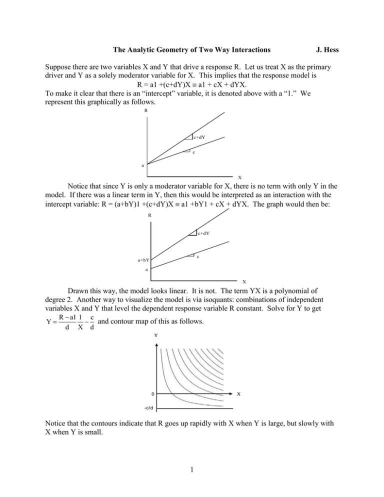
The Analytic Geometry of Two Way Interactions
J. Hess
Suppose there are two variables X and Y that drive a response R. Let us treat X as the primary
driver and Y as a solely moderator variable for X. This implies that the response model is
R = a1 +(c+dY)X  a1 + cX + dYX.
To make it clear that there is an “intercept” variable, it is denoted above with a “1.” We
represent this graphically as follows.
R
c+dY
c
a
X
Notice that since Y is only a moderator variable for X, there is no term with only Y in the
model. If there was a linear term in Y, then this would be interpreted as an interaction with the
intercept variable: R = (a+bY)1 +(c+dY)X  a1 +bY1 + cX + dYX. The graph would then be:
R
c+dY
c
a+bY
a
X
Drawn this way, the model looks linear. It is not. The term YX is a polynomial of
degree 2. Another way to visualize the model is via isoquants: combinations of independent
variables X and Y that level the dependent response variable R constant. Solve for Y to get
Y
R  a1 1 c
 and contour map of this as follows.
d X d
Y
0
X
-c/d
Notice that the contours indicate that R goes up rapidly with X when Y is large, but slowly with
X when Y is small.
1
Also if you move along a ray where Y=kX, the relationship gets progressively steeper since R =
a1 + cX + dkX2.
R
a
X | Y=kX
In the graph below, we see the relationship with all its curvature.
Notice that in the above graphs, it has been implicitly assumed that the coefficients are
R is not the case, there are a wide variety of possible situations to consider as
positive. When this
seen in the table below.
c
d
b
1
+
+
+
2
+
+
–
3
+
–
+
4
+
–
–
5
–
+
+
6
–
+
–
7
–
–
+
8
–
–
–
2
These possibilities lead to the following types of graphs.
R
R
R
X
c
+
1
d
+
X
b
+
c
+
2
R
d
+
b
–
3
d
+
d
–
c
–
6
4
d
+
b
–
c
+
d
–
b
–
c
–
d
–
b
–
R
X
b
+
X
b
+
R
X
5
X
c
+
R
c
–
R
X
c
–
7
d
–
X
b
+
8
If there was a 22 experiment that set X and Y equal to two values, the appearance of the
graphs very much depends on whether the two values lie to the left or right or straddle the point
at which the curves above cross. It also depends on how large the values of Y are taken.
Consider, for example case 1, but suppose that Y is set equal to very negative values so that the
slope of the curves is not even positive (as seen above); this simply requires Y<-c/d. If negative
values of Y that small are allowed, then we could have a graph of case 1 that looks precisely like
case 5 (see below).
R
R
Y 1+  Y
Y 2+  Y
Y1
Y2
X
X1
1
c
+
X
X 1+  X
d
+
X2
b
+
5
c
–
X 2+  X
d
+
b
+
Consider, R=6+Y+(1+Y)X evaluated at Y= -3 and -2 versus R=1+Y+(-4+Y)X evaluated
at Y= 2 and 3. If we did not know the exact values of Y, but just Smaller and Larger, we would
have the identical graph. It would be easy to confuse the negative values of the interaction
variable Y for a negative main effect.
R
4
-1
3
-2
Y=smaller
0
Y=larger
X
3