CIS 313: Analysis and
Design of Algorithms
Chapter 1
Introduction
Copyright © 2007 Pearson Addison-Wesley. All rights reserved.
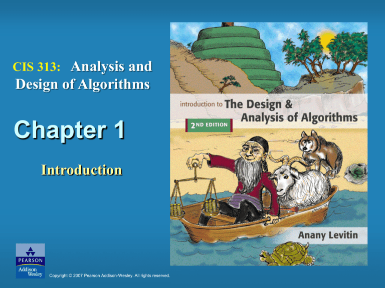
‫لغز‬
‫رجل معه مركب وخروف وذئب وبرسيم‪ ,‬والمركب ال تتسع أال‬
‫للرجل وحاجه من الثالثة ‪ ,‬وخائف عند نقله للبرسيم ‪ ,‬الذئب يأكل‬
‫الخروف‪ ,‬وعند نقله للذئب الخروف يأكل البرسيم‪ ,‬وال يوجد معه‬
‫أي اغراض أخرى ‪,‬كحبل مثالً وال أي شيء فما هو الحل لنقل‬
‫هذه األشياء الى البر الثاني‬
‫الحل‬
‫‪1-1‬‬
‫يأخذ اوال الخروف ويترك الذئب والبرسيم ثم يرجع للشط ويأخذ‬
‫الذئب وهو راجع يأخذ معه الخروف ويتركه ثم يرجع بالبرسيم ثم‬
‫يذهب اخيرا ليأخذ الخروف‬
‫‪A. Levitin “Introduction to the Design & Analysis of Algorithms,” 2nd ed., Ch. 1‬‬
‫‪Copyright © 2007 Pearson Addison-Wesley. All rights reserved.‬‬
What is an algorithm?
An algorithm is a procedure composed of a sequence of
well-defined steps, specified either in a natural
language (a recipe can be regarded as an algorithm),
or in appropriate code or pseudocode.
In these lectures algorithms will be presented in a
simplified pseudocode.
problem
algorithm
input
Copyright © 2007 Pearson Addison-Wesley. All rights reserved.
“computer”
output
A. Levitin “Introduction to the Design & Analysis of Algorithms,” 2nd ed., Ch. 1
1-2
Algorithm

An algorithm is a sequence of unambiguous
instructions for solving a problem, i.e., for
obtaining a required output for any ‘legal ’ input
in a finite amount of time.
• Can be represented various forms
• Unambiguity/clearness
• Effectiveness
• Finiteness/termination
• Correctness
Copyright © 2007 Pearson Addison-Wesley. All rights reserved.
A. Levitin “Introduction to the Design & Analysis of Algorithms,” 2nd ed., Ch. 1
1-3
Historical Perspective

Euclid’s algorithm for finding the greatest common divisor

Muhammad ibn Musa al-Khwarizmi – 9th century
mathematician ‫محمد بن موسى الخوارزمي‬
www.lib.virginia.edu/science/parshall/khwariz.html
Copyright © 2007 Pearson Addison-Wesley. All rights reserved.
A. Levitin “Introduction to the Design & Analysis of Algorithms,” 2nd ed., Ch. 1
1-4
Notion of algorithm and problem
problem
algorithm
input
(or instance)
“computer”
output
algorithmic solution
(different from a conventional solution)
Copyright © 2007 Pearson Addison-Wesley. All rights reserved.
A. Levitin “Introduction to the Design & Analysis of Algorithms,” 2nd ed., Ch. 1
1-5
Review: Induction
 Suppose
• S(k) is true for fixed constant k
– Often k = 0
• S(n)  S(n+1) for all n >= k
 Then
S(n) is true for all n >= k
Copyright © 2007 Pearson Addison-Wesley. All rights reserved.
A. Levitin “Introduction to the Design & Analysis of Algorithms,” 2nd ed., Ch. 1
1-6
Proof By Induction
Claim: S(n) is true for all n >= k
 Basis:

• Show formula is true when n = k

Inductive hypothesis:
• Assume formula is true for an arbitrary n

Step:
• Show that formula is then true for n+1
Copyright © 2007 Pearson Addison-Wesley. All rights reserved.
A. Levitin “Introduction to the Design & Analysis of Algorithms,” 2nd ed., Ch. 1
1-7
Induction Example: Gaussian Closed Form

Prove 1 + 2 + 3 + … + n = n(n+1) / 2
• Basis:
– If n = 0, then 0 = 0(0+1) / 2
• Inductive hypothesis:
– Assume 1 + 2 + 3 + … + n = n(n+1) / 2
• Step (show true for n+1):
1 + 2 + … + n + n+1 = (1 + 2 + …+ n) + (n+1)
= n(n+1)/2 + n+1 = [n(n+1) + 2(n+1)]/2
= (n+1)(n+2)/2 = (n+1)(n+1 + 1) / 2
Copyright © 2007 Pearson Addison-Wesley. All rights reserved.
A. Levitin “Introduction to the Design & Analysis of Algorithms,” 2nd ed., Ch. 1
1-8
Induction Example: Geometric Closed Form
 Prove a0
all a  1
+ a1 + … + an = (an+1 - 1)/(a - 1) for
• Basis: show that a0 = (a0+1 - 1)/(a - 1)
a0 = 1 = (a1 - 1)/(a - 1)
• Inductive hypothesis:
– Assume a0 + a1 + … + an = (an+1 - 1)/(a - 1)
• Step (show true for n+1):
a0 + a1 + … + an+1 = a0 + a1 + … + an + an+1
= (an+1 - 1)/(a - 1) + an+1 = (an+1+1 - 1)/(a - 1)
Copyright © 2007 Pearson Addison-Wesley. All rights reserved.
A. Levitin “Introduction to the Design & Analysis of Algorithms,” 2nd ed., Ch. 1
1-9
Induction
We’ve been using weak induction
 Strong induction also holds

• Basis: show S(0)
• Hypothesis: assume S(k) holds for arbitrary k <= n
• Step: Show S(n+1) follows

Another variation:
• Basis: show S(0), S(1)
• Hypothesis: assume S(n) and S(n+1) are true
• Step: show S(n+2) follows
Copyright © 2007 Pearson Addison-Wesley. All rights reserved.
A. Levitin “Introduction to the Design & Analysis of Algorithms,” 2nd ed., Ch. 1
1-10
Example of computational problem: sorting

Statement of problem:
• Input: A sequence of n numbers <a1, a2, …, an>
• Output: A reordering of the input sequence <a´1, a´2, …, a´n> so
that a´i ≤ a´j whenever i < j

Instance: The sequence < 5, 3, 2, 8, 3 >

Algorithms:
• Selection sort
• Insertion sort
• Merge sort
• (many others)
Copyright © 2007 Pearson Addison-Wesley. All rights reserved.
A. Levitin “Introduction to the Design & Analysis of Algorithms,” 2nd ed., Ch. 1
1-11
Selection Sort

Input: array a[1],…,a[n]

Output: array a sorted in non-decreasing order

Algorithm:
for i=1 to n
swap a[i] with smallest of a[i],…,a[n]
• Is this unambiguous? Effective?
• See also pseudocode, section 3.1
Copyright © 2007 Pearson Addison-Wesley. All rights reserved.
A. Levitin “Introduction to the Design & Analysis of Algorithms,” 2nd ed., Ch. 1
1-12
Some Well-known Computational Problems










Sorting
Searching
Shortest paths in a Graph
Minimum Spanning Tree
Primality testing
Traveling Salesman Problem
Knapsack Problem
Chess
Towers of Hanoi
Program Termination
Some of these problems don’t have efficient algorithms,
or algorithms at all!
Copyright © 2007 Pearson Addison-Wesley. All rights reserved.
A. Levitin “Introduction to the Design & Analysis of Algorithms,” 2nd ed., Ch. 1
1-13
Basic Issues Related to Algorithms

How to design algorithms

How to express algorithms

Proving correctness

Efficiency (or complexity) analysis
• Theoretical analysis
• Empirical analysis

Optimality
Copyright © 2007 Pearson Addison-Wesley. All rights reserved.
A. Levitin “Introduction to the Design & Analysis of Algorithms,” 2nd ed., Ch. 1
1-14
Algorithm design strategies


Brute force
Divide and conquer

Decrease and conquer

Transform and conquer
Copyright © 2007 Pearson Addison-Wesley. All rights reserved.

Greedy approach

Dynamic programming

Backtracking and branch-andbound

Space and time tradeoffs
A. Levitin “Introduction to the Design & Analysis of Algorithms,” 2nd ed., Ch. 1
1-15
Analysis of Algorithms
 How
good is the algorithm?
• Correctness
• Time efficiency
• Space efficiency
 Does
there exist a better algorithm?
• Lower bounds
• Optimality
Copyright © 2007 Pearson Addison-Wesley. All rights reserved.
A. Levitin “Introduction to the Design & Analysis of Algorithms,” 2nd ed., Ch. 1
1-16
What is an algorithm?

1.
Recipe, process, method, technique, procedure, routine,…
with the following requirements:
Finiteness
 terminates after a finite number of steps
2.
Definiteness
 rigorously and unambiguously specified
3.
Clearly specified input
 valid inputs are clearly specified
4.
Clearly specified/expected output
 can be proved to produce the correct output given a valid input
5.
Effectiveness
 steps are sufficiently simple and basic
Copyright © 2007 Pearson Addison-Wesley. All rights reserved.
A. Levitin “Introduction to the Design & Analysis of Algorithms,” 2nd ed., Ch. 1
1-17
Why study algorithms?

Theoretical importance
• the core of computer science

Practical importance
• A practitioner’s toolkit of known algorithms
• Framework for designing and analyzing algorithms for new
problems
Example: Google’s PageRank Technology
Copyright © 2007 Pearson Addison-Wesley. All rights reserved.
A. Levitin “Introduction to the Design & Analysis of Algorithms,” 2nd ed., Ch. 1
1-18
Euclid’s Algorithm
Problem: Find gcd(m,n), the greatest common divisor of two
nonnegative, not both zero integers m and n
Examples: gcd(60,24) = 12,
gcd(60,0) = 60,
gcd(0,0) = ?
Euclid’s algorithm is based on repeated application of equality
gcd(m,n) = gcd(n, m mod n)
until the second number becomes 0, which makes the problem
trivial.
Example: gcd(60,24) = gcd(24,12) = gcd(12,0) = 12
Copyright © 2007 Pearson Addison-Wesley. All rights reserved.
A. Levitin “Introduction to the Design & Analysis of Algorithms,” 2nd ed., Ch. 1
1-19
Two descriptions of Euclid’s algorithm
Step 1 If n = 0, return m and stop; otherwise go to Step 2
Step 2 Divide m by n and assign the value of the remainder to r
Step 3 Assign the value of n to m and the value of r to n. Go to
Step 1.
while n ≠ 0 do
r ← m mod n
m← n
n←r
return m
Copyright © 2007 Pearson Addison-Wesley. All rights reserved.
A. Levitin “Introduction to the Design & Analysis of Algorithms,” 2nd ed., Ch. 1
1-20
Other methods for computing gcd(m,n)
Consecutive integer checking algorithm
Step 1 Assign the value of min{m,n} to t
Step 2 Divide m by t. If the remainder is 0, go to Step 3;
otherwise, go to Step 4
Step 3 Divide n by t. If the remainder is 0, return t and stop;
otherwise, go to Step 4
Step 4 Decrease t by 1 and go to Step 2
Is this slower than Euclid’s algorithm?
How much slower?
O(n), if n <= m , vs O(log n)
Copyright © 2007 Pearson Addison-Wesley. All rights reserved.
A. Levitin “Introduction to the Design & Analysis of Algorithms,” 2nd ed., Ch. 1
1-21
Other methods for gcd(m,n) [cont.]
Middle-school procedure
Step 1
Step 2
Step 3
Step 4
Find the prime factorization of m
Find the prime factorization of n
Find all the common prime factors
Compute the product of all the common prime factors
and return it as gcd(m,n)
Is this an algorithm?
How efficient is it?
Time complexity: O(sqrt(n))
Copyright © 2007 Pearson Addison-Wesley. All rights reserved.
A. Levitin “Introduction to the Design & Analysis of Algorithms,” 2nd ed., Ch. 1
1-22
Sieve of Eratosthenes
Input: Integer n ≥ 2
Output: List of primes less than or equal to n
for p ← 2 to n do A[p] ← p
for p ← 2 to n do
if A[p]  0 //p hasn’t been previously eliminated from the list
j ← p* p
while j ≤ n do
A[j] ← 0 //mark element as eliminated
j←j+p
Example: 2 3 4 5 6 7 8 9 10 11 12 13 14 15 16 17 18 19 20
Time complexity: O(n)
Copyright © 2007 Pearson Addison-Wesley. All rights reserved.
A. Levitin “Introduction to the Design & Analysis of Algorithms,” 2nd ed., Ch. 1
1-23
Two main issues related to algorithms

How to design algorithms

How to analyze algorithm efficiency
Copyright © 2007 Pearson Addison-Wesley. All rights reserved.
A. Levitin “Introduction to the Design & Analysis of Algorithms,” 2nd ed., Ch. 1
1-24
Algorithm design techniques/strategies

Brute force

Greedy approach

Divide and conquer

Dynamic programming

Decrease and conquer

Iterative improvement

Transform and conquer

Backtracking

Space and time tradeoffs

Branch and bound
Copyright © 2007 Pearson Addison-Wesley. All rights reserved.
A. Levitin “Introduction to the Design & Analysis of Algorithms,” 2nd ed., Ch. 1
1-25
Analysis of algorithms

How good is the algorithm?
• time efficiency
• space efficiency
• correctness ignored in this course

Does there exist a better algorithm?
• lower bounds
• optimality
Copyright © 2007 Pearson Addison-Wesley. All rights reserved.
A. Levitin “Introduction to the Design & Analysis of Algorithms,” 2nd ed., Ch. 1
1-26
Important problem types

sorting

searching

string processing

graph problems

combinatorial problems

geometric problems

numerical problems
Copyright © 2007 Pearson Addison-Wesley. All rights reserved.
A. Levitin “Introduction to the Design & Analysis of Algorithms,” 2nd ed., Ch. 1
1-27
Sorting (I)

Rearrange the items of a given list in ascending order.
• Input: A sequence of n numbers <a1, a2, …, an>
• Output: A reordering <a´1, a´2, …, a´n> of the input sequence such that
a´1≤ a´2 ≤ … ≤ a´n.

Why sorting?
• Help searching
• Algorithms often use sorting as a key subroutine.

Sorting key
• A specially chosen piece of information used to guide sorting. E.g., sort
student records by names.
Copyright © 2007 Pearson Addison-Wesley. All rights reserved.
A. Levitin “Introduction to the Design & Analysis of Algorithms,” 2nd ed., Ch. 1
1-28
Sorting (II)

Examples of sorting algorithms
•
•
•
•
•


Selection sort
Bubble sort
Insertion sort
Merge sort
Heap sort …
Evaluate sorting algorithm complexity: the number of key comparisons.
Two properties
•
•
Stability: A sorting algorithm is called stable if it preserves the relative order
of any two equal elements in its input.
In place : A sorting algorithm is in place if it does not require extra memory,
except, possibly for a few memory units.
Copyright © 2007 Pearson Addison-Wesley. All rights reserved.
A. Levitin “Introduction to the Design & Analysis of Algorithms,” 2nd ed., Ch. 1
1-29
Selection Sort
Algorithm SelectionSort(A[0..n-1])
//The algorithm sorts a given array by selection sort
//Input: An array A[0..n-1] of orderable elements
//Output: Array A[0..n-1] sorted in ascending order
for i  0 to n – 2 do
min  i
for j  i + 1 to n – 1 do
if A[j] < A[min]
min  j
swap A[i] and A[min]
Copyright © 2007 Pearson Addison-Wesley. All rights reserved.
A. Levitin “Introduction to the Design & Analysis of Algorithms,” 2nd ed., Ch. 1
1-30
Searching


Find a given value, called a search key, in a given set.
Examples of searching algorithms
• Sequential search
• Binary search …
Input: sorted array a_i < … < a_j and key x;
m (i+j)/2;
while i < j and x != a_m do
if x < a_m then j  m-1
else i  m+1;
if x = a_m then output a_m;
Time: O(log n)
Copyright © 2007 Pearson Addison-Wesley. All rights reserved.
A. Levitin “Introduction to the Design & Analysis of Algorithms,” 2nd ed., Ch. 1
1-31
String Processing



A string is a sequence of characters from an alphabet.
Text strings: letters, numbers, and special characters.
String matching: searching for a given word/pattern in a
text.
Examples:
(i) searching for a word or phrase on WWW or in a
Word document
(ii) searching for a short read in the reference genomic
sequence
Copyright © 2007 Pearson Addison-Wesley. All rights reserved.
A. Levitin “Introduction to the Design & Analysis of Algorithms,” 2nd ed., Ch. 1
1-32
Graph Problems



Informal definition
• A graph is a collection of points called vertices, some of
which are connected by line segments called edges.
Modeling real-life problems
• Modeling WWW
• Communication networks
• Project scheduling …
Examples of graph algorithms
• Graph traversal algorithms
• Shortest-path algorithms
• Topological sorting
Copyright © 2007 Pearson Addison-Wesley. All rights reserved.
A. Levitin “Introduction to the Design & Analysis of Algorithms,” 2nd ed., Ch. 1
1-33
Fundamental data structures

list

graph
• array

tree and binary tree
• linked list

set and dictionary
• string

stack

queue

priority queue/heap
Copyright © 2007 Pearson Addison-Wesley. All rights reserved.
A. Levitin “Introduction to the Design & Analysis of Algorithms,” 2nd ed., Ch. 1
1-34
Linear Data Structures



Arrays
• A sequence of n items of the same
data type that are stored
contiguously in computer memory
and made accessible by specifying a
value of the array’s index.
Linked List
• A sequence of zero or more nodes 
each containing two kinds of
information: some data and one or
more links called pointers to other
nodes of the linked list.
• Singly linked list (next pointer)
• Doubly linked list (next + previous
pointers)
a1
Copyright © 2007 Pearson Addison-Wesley. All rights reserved.
a2
…
Arrays
fixed length (need preliminary
reservation of memory)
contiguous memory locations
direct access
Insert/delete




Linked Lists
dynamic length
arbitrary memory locations
access by following links
Insert/delete




an
.
A. Levitin “Introduction to the Design & Analysis of Algorithms,” 2nd ed., Ch. 1
1-35
Stacks and Queues


Stacks
• A stack of plates
– insertion/deletion can be done only at the top.
– LIFO
• Two operations (push and pop)
Queues
• A queue of customers waiting for services
– Insertion/enqueue from the rear and deletion/dequeue from
the front.
– FIFO
• Two operations (enqueue and dequeue)
Copyright © 2007 Pearson Addison-Wesley. All rights reserved.
A. Levitin “Introduction to the Design & Analysis of Algorithms,” 2nd ed., Ch. 1
1-36
Priority Queue and Heap

Priority queues (implemented using heaps)
A data structure for maintaining a set of elements,
each associated with a key/priority, with the
following operations



Finding the element with the highest priority

Deleting the element with the highest priority

Inserting a new element
9
Scheduling jobs on a shared computer
6
5
8
2
3
9 6 8 5 2 3
Copyright © 2007 Pearson Addison-Wesley. All rights reserved.
A. Levitin “Introduction to the Design & Analysis of Algorithms,” 2nd ed., Ch. 1
1-37
Graphs




Formal definition
• A graph G = <V, E> is defined by a pair of two sets: a
finite set V of items called vertices and a set E of vertex
pairs called edges.
Undirected and directed graphs (digraphs).
What’s the maximum number of edges in an undirected
graph with |V| vertices?
Complete, dense, and sparse graphs
• A graph with every pair of its vertices connected by an
edge is called complete, K|V|
Copyright © 2007 Pearson Addison-Wesley. All rights reserved.
1
2
3
4
A. Levitin “Introduction to the Design & Analysis of Algorithms,” 2nd ed., Ch. 1
1-38
Graph Representation



Adjacency matrix
• n x n boolean matrix if |V| is n.
• The element on the ith row and jth column is 1 if there’s an
edge from ith vertex to the jth vertex; otherwise 0.
• The adjacency matrix of an undirected graph is symmetric.
Adjacency linked lists
• A collection of linked lists, one for each vertex, that contain all
the vertices adjacent to the list’s vertex.
Which data structure would you use if the graph is a 100-node star
shape?
0111
0001
0001
0000
Copyright © 2007 Pearson Addison-Wesley. All rights reserved.
2
4
4
3
4
A. Levitin “Introduction to the Design & Analysis of Algorithms,” 2nd ed., Ch. 1
1-39
Weighted Graphs

Weighted graphs
• Graphs or digraphs with numbers assigned to the edges.
1
6
Copyright © 2007 Pearson Addison-Wesley. All rights reserved.
5
2
9
3
4
8
7
A. Levitin “Introduction to the Design & Analysis of Algorithms,” 2nd ed., Ch. 1
1-40
Graph Properties -- Paths and Connectivity



Paths
• A path from vertex u to v of a graph G is defined as a sequence of
adjacent (connected by an edge) vertices that starts with u and ends
with v.
• Simple paths: All edges of a path are distinct.
• Path lengths: the number of edges, or the number of vertices – 1.
Connected graphs
• A graph is said to be connected if for every pair of its vertices u and
v there is a path from u to v.
Connected component
• The maximum connected subgraph of a given graph.
Copyright © 2007 Pearson Addison-Wesley. All rights reserved.
A. Levitin “Introduction to the Design & Analysis of Algorithms,” 2nd ed., Ch. 1
1-41
Graph Properties -- Acyclicity


Cycle
• A simple path of a positive length that starts and
ends a the same vertex.
Acyclic graph
• A graph without cycles
• DAG (Directed Acyclic Graph)
Copyright © 2007 Pearson Addison-Wesley. All rights reserved.
1
2
3
4
A. Levitin “Introduction to the Design & Analysis of Algorithms,” 2nd ed., Ch. 1
1-42
Trees


Trees
• A tree (or free tree) is a connected acyclic graph.
• Forest: a graph that has no cycles but is not necessarily connected.
Properties of trees
• For every two vertices in a tree there always exists exactly one
simple path from one of these vertices to the other. Why?
– Rooted trees: The above property makes it possible to select an
arbitrary vertex in a free tree and consider it as the root of the
so called rooted tree.
– Levels in a rooted tree.

|E| = |V| - 1
1
3
rooted
3
5
4
2
Copyright © 2007 Pearson Addison-Wesley. All rights reserved.
4
1
5
2
A. Levitin “Introduction to the Design & Analysis of Algorithms,” 2nd ed., Ch. 1
1-43
Rooted Trees (I)





Ancestors
• For any vertex v in a tree T, all the vertices on the simple
path from the root to that vertex are called ancestors.
Descendants
• All the vertices for which a vertex v is an ancestor are said
to be descendants of v.
Parent, child and siblings
• If (u, v) is the last edge of the simple path from the root to
vertex v, u is said to be the parent of v and v is called a child
of u.
• Vertices that have the same parent are called siblings.
Leaves
• A vertex without children is called a leaf.
Subtree
• A vertex v with all its descendants is called the subtree of T
rooted at v.
Copyright © 2007 Pearson Addison-Wesley. All rights reserved.
A. Levitin “Introduction to the Design & Analysis of Algorithms,” 2nd ed., Ch. 1
1-44
Rooted Trees (II)


Depth of a vertex
• The length of the simple path from the root to the vertex.
Height of a tree
• The length of the longest simple path from the root to a leaf.
h=2
3
4
1
5
2
Copyright © 2007 Pearson Addison-Wesley. All rights reserved.
A. Levitin “Introduction to the Design & Analysis of Algorithms,” 2nd ed., Ch. 1
1-45
Ordered Trees




Ordered trees
• An ordered tree is a rooted tree in which all the children of each
vertex are ordered.
Binary trees
• A binary tree is an ordered tree in which every vertex has no more
than two children and each children is designated s either a left child
or a right child of its parent.
Binary search trees
• Each vertex is assigned a number.
• A number assigned to each parental vertex is larger than all the
numbers in its left subtree and smaller than all the numbers in its
right subtree.
log2n  h  n – 1, where h is the height of a binary tree and n the size.
9
6
6
5
8
2
Copyright © 2007 Pearson Addison-Wesley. All rights reserved.
3
3
2
9
5
8
A. Levitin “Introduction to the Design & Analysis of Algorithms,” 2nd ed., Ch. 1
1-46