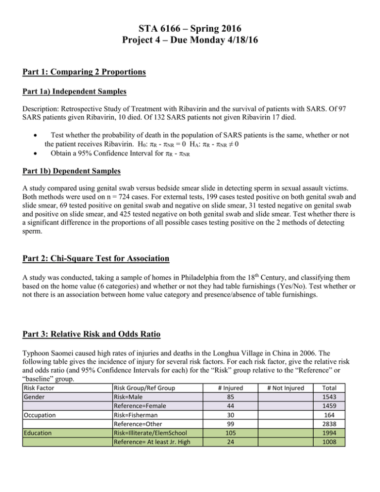
STA 6166 – Spring 2016
Project 4 – Due Monday 4/18/16
Part 1: Comparing 2 Proportions
Part 1a) Independent Samples
Description: Retrospective Study of Treatment with Ribavirin and the survival of patients with SARS. Of 97
SARS patients given Ribavirin, 10 died. Of 132 SARS patients not given Ribavirin 17 died.


Test whether the probability of death in the population of SARS patients is the same, whether or not
the patient receives Ribavirin. H0: R - NR = 0 HA: R - NR ≠ 0
Obtain a 95% Confidence Interval for R - NR
Part 1b) Dependent Samples
A study compared using genital swab versus bedside smear slide in detecting sperm in sexual assault victims.
Both methods were used on n = 724 cases. For external tests, 199 cases tested positive on both genital swab and
slide smear, 69 tested positive on genital swab and negative on slide smear, 31 tested negative on genital swab
and positive on slide smear, and 425 tested negative on both genital swab and slide smear. Test whether there is
a significant difference in the proportions of all possible cases testing positive on the 2 methods of detecting
sperm.
Part 2: Chi-Square Test for Association
A study was conducted, taking a sample of homes in Philadelphia from the 18th Century, and classifying them
based on the home value (6 categories) and whether or not they had table furnishings (Yes/No). Test whether or
not there is an association between home value category and presence/absence of table furnishings.
Part 3: Relative Risk and Odds Ratio
Typhoon Saomei caused high rates of injuries and deaths in the Longhua Village in China in 2006. The
following table gives the incidence of injury for several risk factors. For each risk factor, give the relative risk
and odds ratio (and 95% Confidence Intervals for each) for the “Risk” group relative to the “Reference” or
“baseline” group.
Risk Factor
Gender
Occupation
Education
Risk Group/Ref Group
Risk=Male
Reference=Female
Risk=Fisherman
Reference=Other
Risk=Illiterate/ElemSchool
Reference= At least Jr. High
# Injured
85
44
30
99
105
24
# Not Injured
Total
1543
1459
164
2838
1994
1008
Part 4: Simple Linear Regression
A researcher is interested in the effect of different levels of a nutrient in the feed of mice on
weight gain. She samples 30 mice of a particular breed and assigns them randomly to one of 6
levels of the nutrient (0, 20, 40, 60, 80, 100). There are 5 mice per level. The datasets are
micegrow.xls and micegrow.dat. The response (dependent) variable is weight change over a
3-week period.




Obtain a scatterplot of weight change versus nutrient level
Fit a simple linear regression, relating weight change to nutrient level
Test whether there is a positive association between weight change and nutrient level
Give a 95% confidence interval for the mean change in weight as nutrient level is increased
by 1 unit
 Obtain the analysis of variance table and coefficients of correlation and determination
 Conduct the F-test for Lack of fit
Part 5: Multiple Linear Regression
Description: Regression models for adjusted total costs (Y, millions of $HK)
and average floor area (m^2), total floor area (m^2), average storey height (m)
for 14 Reinforced Concrete (RC) and 23 steel buildings in Hong Kong.
Variables/Columns
Building ID (within type)
7-8
Building Type
16
/* 1=RC, 2=Steel
Average floor area
18-24
Total Floor Area
26-32
Average storey height
36-40
Adjusted Construction Cost
42-48
*/
 Fit a multiple linear regression model, relating cost Y to the 3 numeric predictors: average
floor area, total floor area, and average storey height and a dummy variable for Steel
Buildings. Give the estimated regression equation
 Obtain the actual and predicted cost for each building
 Obtain the analysis of variance and test whether any of the predictors are associated with
sale price (=0.05):
H0: 1=…=4 = 0 HA: Not all s are 0
 State which (if any) of the individual partial regression coefficients are significant at the
=0.05 significance level (controlling for all other variables).
 Fit a model with all interactions between steel type and each of the 3 predictors. Test
whether the interaction effects are all 0 simultaneously at the =0.05 significance level using
the method COMPARING REGRESSION MODELS on slides 10 and 11 of Chapter 12.
 What proportion of the variation in Costs is “explained by each model?