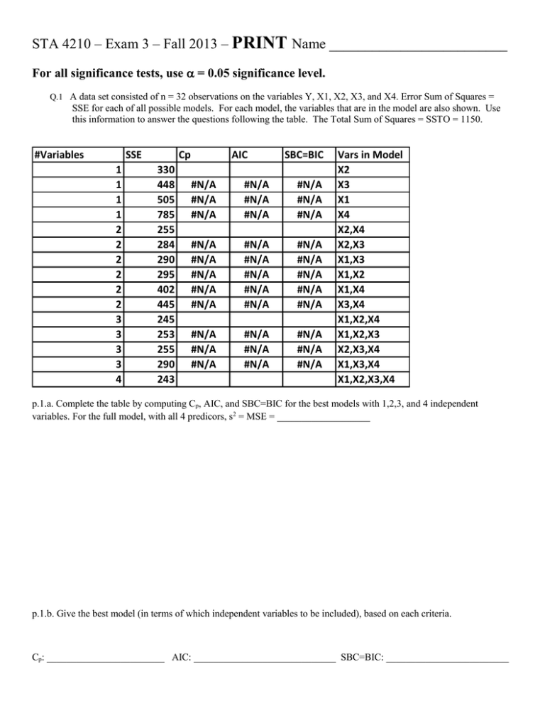
STA 4210 – Exam 3 – Fall 2013 – PRINT Name _________________________
For all significance tests, use  = 0.05 significance level.
Q.1 A data set consisted of n = 32 observations on the variables Y, X1, X2, X3, and X4. Error Sum of Squares =
SSE for each of all possible models. For each model, the variables that are in the model are also shown. Use
this information to answer the questions following the table. The Total Sum of Squares = SSTO = 1150.
#Variables
SSE
1
1
1
1
2
2
2
2
2
2
3
3
3
3
4
Cp
330
448
505
785
255
284
290
295
402
445
245
253
255
290
243
AIC
SBC=BIC
#N/A
#N/A
#N/A
#N/A
#N/A
#N/A
#N/A
#N/A
#N/A
#N/A
#N/A
#N/A
#N/A
#N/A
#N/A
#N/A
#N/A
#N/A
#N/A
#N/A
#N/A
#N/A
#N/A
#N/A
#N/A
#N/A
#N/A
#N/A
#N/A
#N/A
#N/A
#N/A
#N/A
Vars in Model
X2
X3
X1
X4
X2,X4
X2,X3
X1,X3
X1,X2
X1,X4
X3,X4
X1,X2,X4
X1,X2,X3
X2,X3,X4
X1,X3,X4
X1,X2,X3,X4
p.1.a. Complete the table by computing Cp, AIC, and SBC=BIC for the best models with 1,2,3, and 4 independent
variables. For the full model, with all 4 predicors, s2 = MSE = ___________________
p.1.b. Give the best model (in terms of which independent variables to be included), based on each criteria.
Cp: ________________________ AIC: _____________________________ SBC=BIC: _________________________
Q.2. An analysis relating Height to 6 body length attributes in n=33 female police officer applicants was conducted. The 6
attributes (predictors) were: Upper Arm, Lower Arm, Hand, Upper Leg, Lower Leg, Foot. Three models were fit.
Model 1: E H    0  UAUA   LA LA   H H  ULUL   LL LL   F F
SSR1  568 SSE1  198
Model 2: E H    0  ULUL   LL LL   F F
SSR2  551 SSE2  215
Model 3: E H    0   LL LL   F F
SSR3  532 SSE3  234
p.2.a. Use Model 1 to test H 0 : UA   LA   H  UL   LL   F  0
Test Statistic: ___________________ Rejection Region: ______________________ Reject H0: Yes / No
p.2.b. The regression coefficient estimates, and standard errors are given below. Controlling for all other predictors in the
3 models, circle which of the predictors are significant at the 0.05 level:
Model 1
UA LA H UL LL F
Model1 Coefficients
Standard Error
Intercept
70.32
12.34
upparm
-0.31
0.47
forearm
0.77
0.61
hand
0.28
0.78
uppleg
0.68
0.42
lowleg
0.84
0.50
foot
2.39
0.94
t Stat
5.70
-0.67
1.26
0.36
1.63
1.69
2.53
P-value
0.0000
0.5102
0.2172
0.7238
0.1157
0.1025
0.0177
Model 2
Model2 Coefficients
Standard Error
Intercept
77.45
10.50
uppleg
0.52
0.33
lowleg
1.19
0.36
foot
2.75
0.84
UL LL F
t Stat
7.38
1.61
3.26
3.28
P-value
0.0000
0.1184
0.0028
0.0027
Model 3
LL F
Model3 Coefficients
Standard Error
Intercept
84.49
9.80
lowleg
1.63
0.25
foot
2.29
0.81
t Stat
8.62
6.65
2.83
P-value
0.0000
0.0000
0.0082
p.2.c. Obtain 95% Confidence Intervals for  LL for models 1,2, and3 (do not make Bonferroni adjustments).
Model 1 _____________________ Model 2 ____________________ Model 3 ________________________
p.2.d. This is best described as an example of : a) autocorrelation
b) multicollinearity
c) outlying observation
p.2.e. Use models 1 and 3 to test whether after controlling for Lower Leg and Foot, none of the remaining predictors are
associated with Height. H 0 : UA   LA   H  UL  0
Test Statistic: ___________________ Rejection Region: ______________________ Reject H0: Yes / No
Q.3. A study related building costs (Y) for skyscrapers in Hong Kong to 4 factors: Steel (X1 = 1 if Yes, 0 if Reinforced
Concrete), Average Floor Area (X2), Total Floor Area (X3), and Average Story Height (X4). Consider the model:
E Y   0  1 X1  2 X 2  3 X 3  4 X 4
p.3.a. Complete the table
ANOVA
df
Regression
Residual
Total
Intercept
Steel
AvFloorK
TotFlr10K
StryHt
SS
8.7009
MS
F
F(.95)
8.7334
Coefficients
Standard Error t Stat
-0.3691
0.1532
-2.4097
0.0197
0.0110
0.3415
0.0297
0.0922
0.0048
19.3026
0.0998
0.0419
2.3801
t(.975)
p.3.b. Give the predicted cost for a building built of Steel, with AvFloorK = 2.0, TotFlr10K = 7.0, and StoryHt = 4.0.
p.3.c. Give a 95% confidence interval for the difference in Steel and Reinforced Concrete, controlling for all other
predictors.
p.3.d. What proportion of the variation in cost is “explained” by the regression model?
Q.4. A regression model was fit for a municipal trolley company, relating the number of passengers (Y, in 1000s) to
number of miles per week (X, in 1000s) for a period of n=20 weeks. The model and residuals are given below.
week(t)
1
2
3
4
5
6
7
8
9
10
11
12
13
14
15
16
17
18
19
20
miles_k
pass_k
Y-hat(t)
2.632
18.764
13.51
1.211
6.688
7.93
2.604
16.504
13.40
4.039
22.944
19.03
5.047
25.063
22.99
5.313
20.897
24.03
6.916
30.357
30.33
8.621
27.076
37.02
8.351
28.26
35.96
10.089
36.683
42.79
10.583
40.09
44.73
10.895
39.04
45.95
11.309
45.35
47.58
10.832
51.648
45.70
11.563
58.598
48.57
12.128
55.163
50.79
12.789
57.519
53.39
14.154
52.82
58.75
14.649
59.219
60.69
14.371
70.065
59.60
sum
e(t)
(e(t)-e(t-1))^2t e(t)*e(t-1)
5.26
0.00
0.00
-1.24
42.20
-6.52
3.11
18.89
-3.85
3.91
0.65
12.15
2.07
3.38
8.11
-3.14
27.15
-6.50
0.03
10.02
-0.09
-9.95
99.51
-0.28
-7.70
5.04
76.62
-6.10
2.56
47.02
-4.64
2.15
28.30
-6.91
5.18
32.05
-2.23
21.94
15.39
5.94
66.76
-13.24
10.02
16.64
59.57
4.37
31.96
43.80
4.13
0.06
18.05
-5.93
101.18
-24.49
-1.47
19.85
8.73
10.46
142.51
-15.41
0.00
617.63
279.42
ANOVA
df
Regression
Residual
Total
Intercept
miles_k
1
18
19
SS
5159.89
656.81
5816.70
MS
5159.89
36.49
F
141.41
Significance F
0.000
Coefficients
Standard Error t Stat
P-value
3.17
3.24
0.98
0.340
3.93
0.33
11.89
0.000
p.4.a. Conduct the Durbin-Watson Test for autocorrelated errors (Note: for n=20, p-1=1, =0.05: dL=1.20, dU=1.41):
Test Statistic: __________________ Conclude: Autocorrelation Present
No autocorrelation
p.4.b. Compute the estimate of the autocorrelation parameter used in the Cochrane-Orcutt method.
Withhold judgment
Q.5. A linear regression model is fit, relating the monthly rental price of apartments (Y, in $100s) of similar ages to their
square footage (X1, in 100s ft2), for apartments in three neighborhoods (A,B, and C). The analyst included 2 dummy
variables: (X2=1 if neighborhood A, 0 otherwise) and (X3=1 if neighborhood B, 0 otherwise). She sampled 10 apartments
at random from each neighborhood. She fit 3 models (note, this is an expensive city):
Model 1: E Y    0  1 X 1
Model 2: E Y    0  1 X 1   2 X 2  3 X 3
Model 3: E Y    0  1 X 1   2 X 2  3 X 3   4 X 1 X 2  5 X 1 X 3
The ANOVA table for each model is given below.
ANOVA
Model1
df
Regression
1
Residual
28
Total
29
ANOVA
SS
MS
1448.0 1448.0
152.2
5.4
1600.2
F
266.4
Model2
df
Regression
3
Residual
26
Total
29
ANOVA
SS
1569.1
31.1
1600.2
MS
523.0
1.2
F
437.8
Model3
df
Regression
5
Residual
24
Total
29
SS
1571.4
28.8
1600.2
MS
314.3
1.2
F
262.0
p.5.a. Based on models 2 and 3, test whether there is an interaction between neighborhood and “square footage effect,”
that is, test H0: .
Test Statistic: ______________________________ Rejection Region: ____________________________________
p.5.b. Assuming you failed to find an interaction, use models 1 and 2 to test whether there is a neighborhood effect,
that is, test H0: .
Test Statistic: ______________________________ Rejection Region: ____________________________________
p.5.c. The Regression coefficients for model 2 are given below. Give the fitted equation, relating price ($100s) to square
footage (X1, 100s ft2) for each neighborhood.
Intercept
X1
X2
X3
Coefficients
Standard Error
3.70
0.71
1.48
0.05
2.10
0.49
-2.92
0.50
Neighborhood A:
Neighborhood B:
Neighborhood C:
Critical Values for t, 2, and F Distributions
F Distributions Indexed by Numerator Degrees of Freedom
CDF - Lower tail probabilities
df |
1
2
3
4
5
6
7
8
9
10
11
12
13
14
15
16
17
18
19
20
21
22
23
24
25
26
27
28
29
30
40
50
60
70
80
90
100
110
120
130
140
150
160
170
180
190
200

|
|
|
|
|
|
|
|
|
|
|
|
|
|
|
|
|
|
|
|
|
|
|
|
|
|
|
|
|
|
|
|
|
|
|
|
|
|
|
|
|
|
|
|
|
|
|
|
t.95
6.314
2.920
2.353
2.132
2.015
1.943
1.895
1.860
1.833
1.812
1.796
1.782
1.771
1.761
1.753
1.746
1.740
1.734
1.729
1.725
1.721
1.717
1.714
1.711
1.708
1.706
1.703
1.701
1.699
1.697
1.684
1.676
1.671
1.667
1.664
1.662
1.660
1.659
1.658
1.657
1.656
1.655
1.654
1.654
1.653
1.653
1.653
1.645
t.975
 .295
F.95,1
F.95,2
F.95,3
F.95,4
F.95,5
F.95,6
F.95,7
F.95,8
12.706
4.303
3.182
2.776
2.571
2.447
2.365
2.306
2.262
2.228
2.201
2.179
2.160
2.145
2.131
2.120
2.110
2.101
2.093
2.086
2.080
2.074
2.069
2.064
2.060
2.056
2.052
2.048
2.045
2.042
2.021
2.009
2.000
1.994
1.990
1.987
1.984
1.982
1.980
1.978
1.977
1.976
1.975
1.974
1.973
1.973
1.972
1.960
3.841
5.991
7.815
9.488
11.070
12.592
14.067
15.507
16.919
18.307
19.675
21.026
22.362
23.685
24.996
26.296
27.587
28.869
30.144
31.410
32.671
33.924
35.172
36.415
37.652
38.885
40.113
41.337
42.557
43.773
55.758
67.505
79.082
90.531
101.879
113.145
124.342
135.480
146.567
157.610
168.613
179.581
190.516
201.423
212.304
223.160
233.994
---
161.448
18.513
10.128
7.709
6.608
5.987
5.591
5.318
5.117
4.965
4.844
4.747
4.667
4.600
4.543
4.494
4.451
4.414
4.381
4.351
4.325
4.301
4.279
4.260
4.242
4.225
4.210
4.196
4.183
4.171
4.085
4.034
4.001
3.978
3.960
3.947
3.936
3.927
3.920
3.914
3.909
3.904
3.900
3.897
3.894
3.891
3.888
3.841
199.500
19.000
9.552
6.944
5.786
5.143
4.737
4.459
4.256
4.103
3.982
3.885
3.806
3.739
3.682
3.634
3.592
3.555
3.522
3.493
3.467
3.443
3.422
3.403
3.385
3.369
3.354
3.340
3.328
3.316
3.232
3.183
3.150
3.128
3.111
3.098
3.087
3.079
3.072
3.066
3.061
3.056
3.053
3.049
3.046
3.043
3.041
2.995
215.707
19.164
9.277
6.591
5.409
4.757
4.347
4.066
3.863
3.708
3.587
3.490
3.411
3.344
3.287
3.239
3.197
3.160
3.127
3.098
3.072
3.049
3.028
3.009
2.991
2.975
2.960
2.947
2.934
2.922
2.839
2.790
2.758
2.736
2.719
2.706
2.696
2.687
2.680
2.674
2.669
2.665
2.661
2.658
2.655
2.652
2.650
2.605
224.583
19.247
9.117
6.388
5.192
4.534
4.120
3.838
3.633
3.478
3.357
3.259
3.179
3.112
3.056
3.007
2.965
2.928
2.895
2.866
2.840
2.817
2.796
2.776
2.759
2.743
2.728
2.714
2.701
2.690
2.606
2.557
2.525
2.503
2.486
2.473
2.463
2.454
2.447
2.441
2.436
2.432
2.428
2.425
2.422
2.419
2.417
2.372
230.162
19.296
9.013
6.256
5.050
4.387
3.972
3.687
3.482
3.326
3.204
3.106
3.025
2.958
2.901
2.852
2.810
2.773
2.740
2.711
2.685
2.661
2.640
2.621
2.603
2.587
2.572
2.558
2.545
2.534
2.449
2.400
2.368
2.346
2.329
2.316
2.305
2.297
2.290
2.284
2.279
2.274
2.271
2.267
2.264
2.262
2.259
2.214
233.986
19.330
8.941
6.163
4.950
4.284
3.866
3.581
3.374
3.217
3.095
2.996
2.915
2.848
2.790
2.741
2.699
2.661
2.628
2.599
2.573
2.549
2.528
2.508
2.490
2.474
2.459
2.445
2.432
2.421
2.336
2.286
2.254
2.231
2.214
2.201
2.191
2.182
2.175
2.169
2.164
2.160
2.156
2.152
2.149
2.147
2.144
2.099
236.768
19.353
8.887
6.094
4.876
4.207
3.787
3.500
3.293
3.135
3.012
2.913
2.832
2.764
2.707
2.657
2.614
2.577
2.544
2.514
2.488
2.464
2.442
2.423
2.405
2.388
2.373
2.359
2.346
2.334
2.249
2.199
2.167
2.143
2.126
2.113
2.103
2.094
2.087
2.081
2.076
2.071
2.067
2.064
2.061
2.058
2.056
2.010
238.883
19.371
8.845
6.041
4.818
4.147
3.726
3.438
3.230
3.072
2.948
2.849
2.767
2.699
2.641
2.591
2.548
2.510
2.477
2.447
2.420
2.397
2.375
2.355
2.337
2.321
2.305
2.291
2.278
2.266
2.180
2.130
2.097
2.074
2.056
2.043
2.032
2.024
2.016
2.010
2.005
2.001
1.997
1.993
1.990
1.987
1.985
1.938
|
|
|
|
|
|
|
|
|
|
|
|
|
|
|
|
|
|
|
|
|
|
|
|
|
|
|
|
|
|
|
|
|
|
|
|
|
|
|
|
|
|
|
|
|
|
|
|