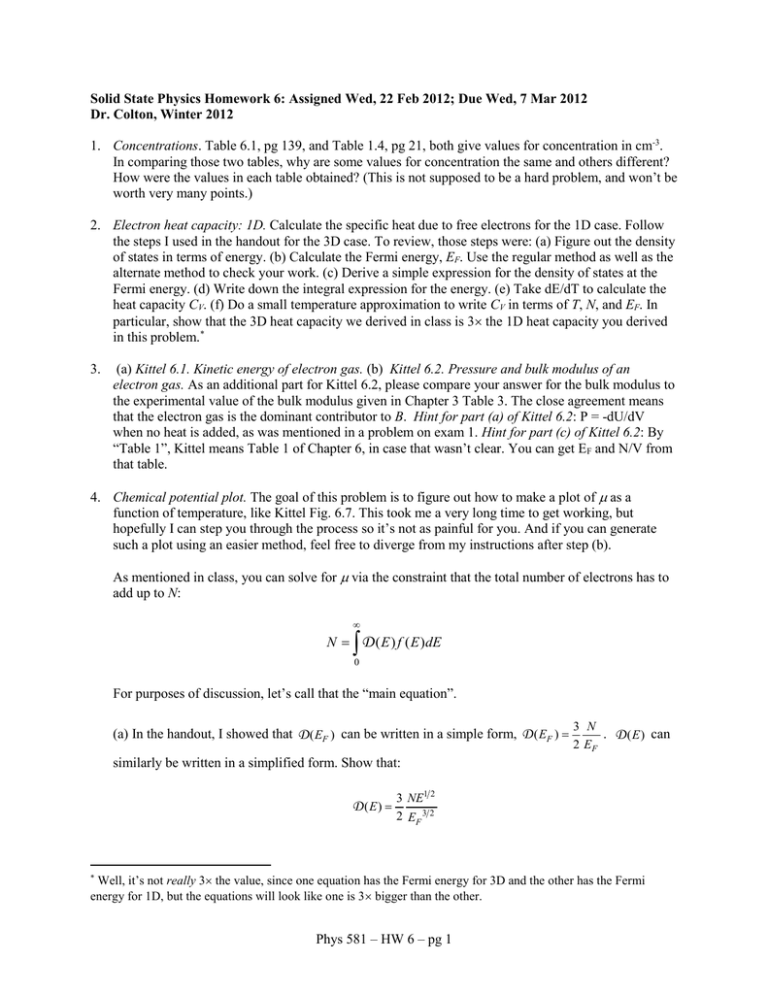
Solid State Physics Homework 6: Assigned Wed, 22 Feb 2012; Due Wed, 7 Mar 2012
Dr. Colton, Winter 2012
1. Concentrations. Table 6.1, pg 139, and Table 1.4, pg 21, both give values for concentration in cm-3.
In comparing those two tables, why are some values for concentration the same and others different?
How were the values in each table obtained? (This is not supposed to be a hard problem, and won’t be
worth very many points.)
2. Electron heat capacity: 1D. Calculate the specific heat due to free electrons for the 1D case. Follow
the steps I used in the handout for the 3D case. To review, those steps were: (a) Figure out the density
of states in terms of energy. (b) Calculate the Fermi energy, EF. Use the regular method as well as the
alternate method to check your work. (c) Derive a simple expression for the density of states at the
Fermi energy. (d) Write down the integral expression for the energy. (e) Take dE/dT to calculate the
heat capacity CV. (f) Do a small temperature approximation to write CV in terms of T, N, and EF. In
particular, show that the 3D heat capacity we derived in class is 3 the 1D heat capacity you derived
in this problem.*
3.
(a) Kittel 6.1. Kinetic energy of electron gas. (b) Kittel 6.2. Pressure and bulk modulus of an
electron gas. As an additional part for Kittel 6.2, please compare your answer for the bulk modulus to
the experimental value of the bulk modulus given in Chapter 3 Table 3. The close agreement means
that the electron gas is the dominant contributor to B. Hint for part (a) of Kittel 6.2: P = -dU/dV
when no heat is added, as was mentioned in a problem on exam 1. Hint for part (c) of Kittel 6.2: By
“Table 1”, Kittel means Table 1 of Chapter 6, in case that wasn’t clear. You can get EF and N/V from
that table.
4. Chemical potential plot. The goal of this problem is to figure out how to make a plot of  as a
function of temperature, like Kittel Fig. 6.7. This took me a very long time to get working, but
hopefully I can step you through the process so it’s not as painful for you. And if you can generate
such a plot using an easier method, feel free to diverge from my instructions after step (b).
As mentioned in class, you can solve for  via the constraint that the total number of electrons has to
add up to N:


N  D ( E ) f ( E )dE
0
For purposes of discussion, let’s call that the “main equation”.
(a) In the handout, I showed that D ( EF ) can be written in a simple form, D ( EF ) 
3 N
.
2 EF
D ( E ) can
similarly be written in a simplified form. Show that:
D (E) 
3 NE1 2
2 EF 3 2
Well, it’s not really 3 the value, since one equation has the Fermi energy for 3D and the other has the Fermi
energy for 1D, but the equations will look like one is 3 bigger than the other.
*
Phys 581 – HW 6 – pg 1
(b) The next step is to get the main equation into a dimensionless form that is easier to work with. Do
a substitution of variables to match Kittel’s plot: x = kT/EF and y = /EF. Also make a dimensionless
substitution for the variable of integration: s = E/EF. Show that when you do that, the main equation
turns into this:

1
2
s2
  ( s  y )/ x
ds
3 0e
1
(c) That is now a fairly simple equation that in principle you could use to solve (numerically) for y,
given a particular value of x. Or equivalently, for a given value of T, you could solve for .
Mathematica can actually do that integral, so I recommend you do that. You may have to use the
“Assuming” command to tell Mathematica that x > 0. It will give you the answer in terms of a
“polylog” function. The integral must have a real answer for our case, but in general the polylog
function can be complex. Due to that and small Mathematica rounding errors, if you actually evaluate
the polylog function here it will return a very tiny imaginary component. That’s not correct, so define
the right-hand side of your main equation to be a function which is just the real part of the result of
the integral. Use the Re[ ] command:
f[x_, y_] = Re[ result of integral that includes polylog ]
(d) You can use the FindRoot command to numerically solve equations in Mathematica. For example,
FindRoot[Sin[y] y/2,{y,2}]
will tell you what the value of y needs to be to have sin(y) be equal to y/2. (Try it.) The {y,2} in the
command just specifies that the computer should begin its search for equality around y = 2. Also note
that there are two equal signs in a row after Sin[y] in the command.
In your case, you can find the y-value that, for example, corresponds to x = 0.3 by using the command
like this:
FindRoot[2/3  f[.3,y],{y,1}]
Play around with the FindRoot command long enough to verify that you are in fact getting values that
match the figure in Kittel. Success! (Careful: as noted in the figure caption, Kittel uses a strange
rescaling of x and y. So the vertical line where kBT = 1 on his graph actually corresponds to x = 0.763
on your graph. Same thing for the horizontal line where  = 1. I have no idea why he uses that factor
of 0.763; it seems very odd to me.)
(e) Getting FindRoot to generate a plot turns out to be a little bit trickier than just looking at answers
for specific values of x, since FindRoot returns the numerical results in a strange format using an
arrow. But you can get around that by defining the function a specific way. In our sin(y) = y/2
example above, for example, suppose you want to determine what y needs to be for an arbitrary
denominator specified by x, not just for a denominator of 2. You can define y to be a function of x via
the results of the FindRoot command, like this:
y[x_] := y/.FindRoot[ Sin[y] y/x,{y,2}]
Phys 581 – HW 6 – pg 2
Typing in y[2] now returns the same result as did the first FindRoot command above. (Try it.) You
can use that y(x) the way you would any other function, including to make a plot for a range of x’s:
Plot[y[x],{x,1.4,3}]
Using a similar technique you can define your rescaled chemical potential y as a function of your
rescaled temperature x.
Finally, even after I got the function properly defined, I still had some trouble with the plot. This was
due to two reasons: (1) something goes to infinity when x = 0 and the program can’t handle it, and (2)
Mathematica defaults to a very large number of points to make graphs look nice so the graph takes a
very, very long time to produce (if at all). Fix the first one by starting your x-axis at x = 0.001 instead
of x = 0. Fix the second one by forcing Mathematica to plot just a limited number of points using the
“MaxRecursion” and “PlotPoints” specifiers. For example, you can type in this command to see a
parabola plotted by connecting lines between only 6 points.
Plot[x^2,{x,0,6},MaxRecursion0,PlotPoints6]
By setting PlotPoints equal to 50 in this manner, I was finally able to get a plot of  vs T that exactly
matches Kittel’s plot. Do the same.
As a final note, there is a complicated technique called the “Sommerfeld expansion” which can be
used to give an equation for the chemical potential that is valid for small temperatures. In terms of our
2 2 4 4
dimensionless variables it is: y  1 
x 
x  ... See http://en.wikipedia.org/wiki/Fermi_gas. If
12
80
you’re curious, the technique is presented with some detail in An Introduction to Thermal Physics by
Daniel Schroeder, chapter 7, pp 282-284. That expansion agrees fairly well with our more accurate
numerical calculation out to about x = 0.5.
5. Kittel 6.3. Chemical potential in two dimensions. Even though as the last problem showed it’s nearly
impossible to get an equation for (T) in three dimensions, it’s relatively easy to obtain such an
equation in the 2D case. Solve this problem using the same “main equation” from the last problem.
6. Kittel 6.5. Liquid He3.
7. Kittel 6.6. Frequency dependence of the electrical conductivity. Hint: assume v = v0e-it. This is a way
of representing sinusoidal oscillations, where it’s understood to get the real information, one must
take the “real part” of the quantities of interest. If you make that assumption, then the given equation
lets you solve for v in terms of the electric field. You should then be able to figure out what is  in
terms of the electric field.
8. Kittel 6.9. Static magnetoconductivity tensor. Hint: it’s static, so the time derivatives are zero. Move
all the velocities to the left hand side, write velocities in terms of j’s (equation 42), then you can write
as a 33 matrix equation. From there you can use e.g. Mathematica to find the inverse of the matrix.
Phys 581 – HW 6 – pg 3