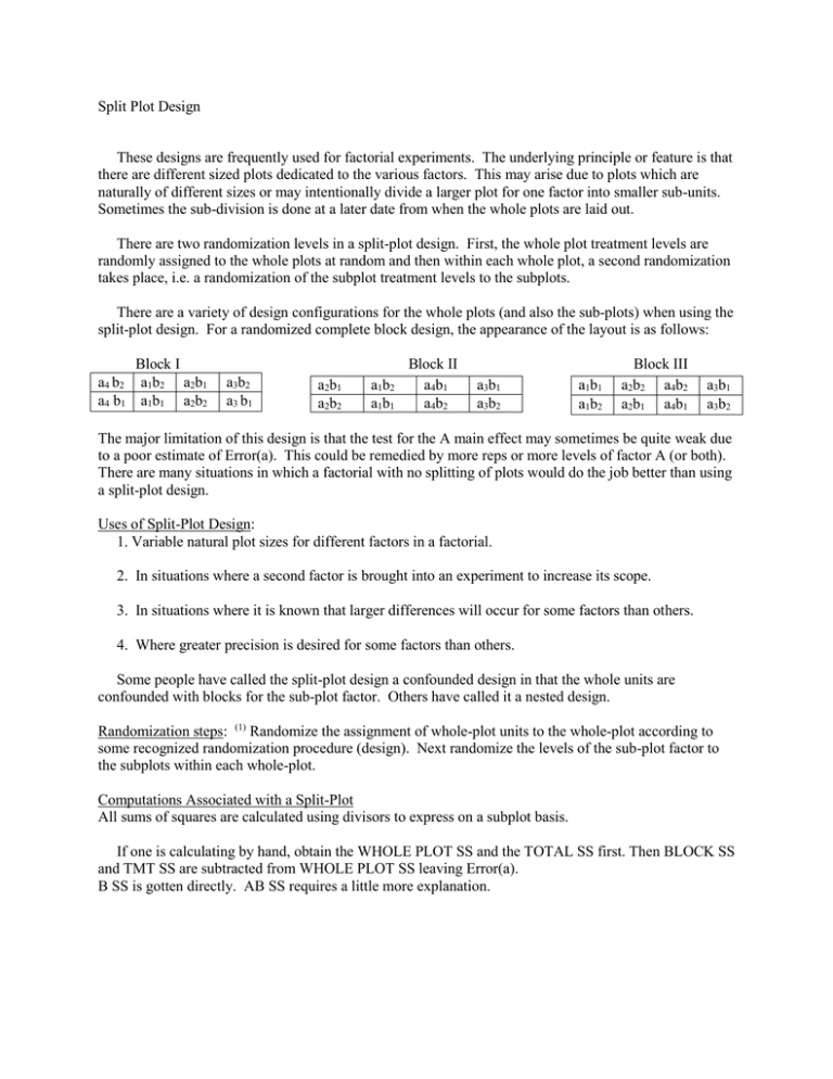
Split Plot Design
These designs are frequently used for factorial experiments. The underlying principle or feature is that
there are different sized plots dedicated to the various factors. This may arise due to plots which are
naturally of different sizes or may intentionally divide a larger plot for one factor into smaller sub-units.
Sometimes the sub-division is done at a later date from when the whole plots are laid out.
There are two randomization levels in a split-plot design. First, the whole plot treatment levels are
randomly assigned to the whole plots at random and then within each whole plot, a second randomization
takes place, i.e. a randomization of the subplot treatment levels to the subplots.
There are a variety of design configurations for the whole plots (and also the sub-plots) when using the
split-plot design. For a randomized complete block design, the appearance of the layout is as follows:
Block I
a4 b2 a1b2 a2b1
a4 b1 a1b1 a2b2
a3b2
a3 b1
a2b1
a2b2
a1b2
a1b1
Block II
a4b1
a4b2
a3b1
a3b2
a1b1
a1b2
Block III
a2b2 a4b2
a2b1 a4b1
a3b1
a3b2
The major limitation of this design is that the test for the A main effect may sometimes be quite weak due
to a poor estimate of Error(a). This could be remedied by more reps or more levels of factor A (or both).
There are many situations in which a factorial with no splitting of plots would do the job better than using
a split-plot design.
Uses of Split-Plot Design:
1. Variable natural plot sizes for different factors in a factorial.
2. In situations where a second factor is brought into an experiment to increase its scope.
3. In situations where it is known that larger differences will occur for some factors than others.
4. Where greater precision is desired for some factors than others.
Some people have called the split-plot design a confounded design in that the whole units are
confounded with blocks for the sub-plot factor. Others have called it a nested design.
Randomization steps: (1) Randomize the assignment of whole-plot units to the whole-plot according to
some recognized randomization procedure (design). Next randomize the levels of the sub-plot factor to
the subplots within each whole-plot.
Computations Associated with a Split-Plot
All sums of squares are calculated using divisors to express on a subplot basis.
If one is calculating by hand, obtain the WHOLE PLOT SS and the TOTAL SS first. Then BLOCK SS
and TMT SS are subtracted from WHOLE PLOT SS leaving Error(a).
B SS is gotten directly. AB SS requires a little more explanation.
A
a1
a2
Form AB table
b1
B
b2
SS AB = SS for Table – CF – SSA – SSB
Same idea would apply if we were calculating a 3-factor interaction.
SS ABC = SS for Table – SSA – SSB – SSAB – SSAC – SSBC.
Error(b) SS is by difference Total SS – Whole plot SS – SSB – SSAB
One has to be very careful in all of this not to make any errors as they tend to affect those effects
obtained by difference.
Using SAS, the procedures would be exactly as one would use with a factorial experiment except the
model would be different.
PROC ANOVA or PROC GLM;
CLASS REP A B;
MODEL Y= REP A REP*A B A*B;
MEANS A|B;
Note that we have introduced a new term REP*A into the model which we didn’t pull out with a factorial
experiment.
With the SAS approach, we could need to test A with REP*A and this will take a separate statement:
TEST H = A / E=REP*A;
The tests of B and AB will be performed correctly using the default error term.
INTERPRETATION OF RESULTS
In general, the interpretation process is very similar to that of a factorial without the splitting. However,
there are some unique features.
First, one would test the A-main effect with the Error(a).
Second, the standard errors for comparing interaction means are different when we are comparing 2 A’s
within a B than 2 B’s within an A. One has to be very careful about this. It is often done wrong is
practice.
The other point is that when there are more than 2-levels of the factors, the interpretation would depend
upon whether each factor is qualitative or quantitative just as it does with any factorial experiment.