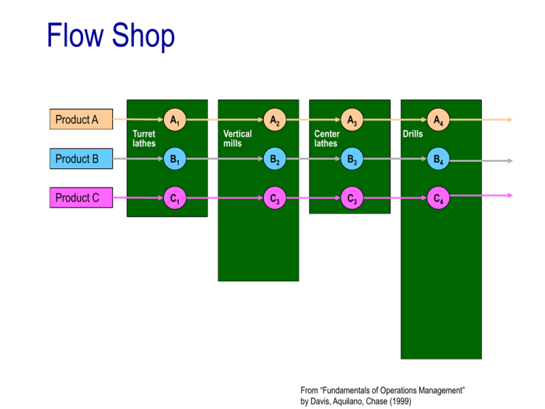
Flow Shop
Product A
A1
Turret
lathes
A2
Vertical
mills
A3
Center
lathes
A4
Drills
Product B
B1
B2
B3
B4
Product C
C1
C3
C3
C4
From “Fundamentals of Operations Management”
by Davis, Aquilano, Chase (1999)
Job Shop
Product A
Product B
A1
A2
Turret
lathes
Vertical
mills
C2
A3
Center
lathes
B1
C3
Drills
B5
Shapers
A4
B2
B4
Grinders
Product C
C1
A5
B3
Horizontal
mills
C4
From “Fundamentals of Operations Management”
by Davis, Aquilano, Chase (1999)
Complexity
m=3
m=2
n=3
n=2
NP-hard
Polynomially
solvable
Job Shop: Two Machines
Consider now problem J2| |Cmax.
The set of jobs N={1,…,n} can be split into two subsets:
NAB - the jobs that consist of two operations with the processing route (A, B)
NBA - the jobs that consist of two operations with the processing route (B, A)
The algorithm presented below is due to R. Jackson (1956).
Jackson's Algorithm
1. Run Johnson's algorithm with the set of jobs NAB and find the corresponding sequence RAB.
2. Run Johnson's algorithm with the set of jobs NBA and find the corresponding sequence RBA.
3. On machine A, first schedule NAB according to RAB and then NBA according to RBA.
4. On machine B, first schedule NBA according to RBA and then NAB according to RAB.
A
B
NAB
NBA
NBA
NAB
Job Shop: Two Machines
Example
Consider Problem J2| |Cmax
j
aj
1
3
2
2
3
1
4
1
5
2
6
4
7
3
bj
2
1
2
1
4
8
9
8
1
9
2
10
11
2
1
Job Shop: Disjunctive Graph Model
Machine
Jobs sequence Processing times
1
2
3
1, 2, 3
p11=10, p21=8, p31=4
2, 1, 4, 3 p12=3, p22=8, p32=6, p42=5
1, 2, 4
p13=4, p23=7, p43=3
p11
Job 1
p21
1,1
2,1
p22
S
3,1
1,2
1,3
p13
p32
3,2
p42
4,2
p12
Job 2 2,2
Job 3
p31
2,3
p23
4,3
p43
T
Job Shop: Disjunctive Graph Model
Machine
Jobs sequence Processing times
1
2
3
1, 2, 3
p11=10, p21=8, p31=4
2, 1, 4, 3 p12=3, p22=8, p32=6, p42=5
1, 2, 4
p13=4, p23=7, p43=3
p11
p21
1,1
2,1
p22
S
3,1
1,2
2,2
p13
p32
3,2
p42
4,2
p12
1,3
p31
2,3
p23
4,3
p43
T
Job Shop: Disjunctive Graph Model
Machine
Jobs sequence Processing times
1
2
3
1, 2, 3
p11=10, p21=8, p31=4
2, 1, 4, 3 p12=3, p22=8, p32=6, p42=5
1, 2, 4
p13=4, p23=7, p43=3
p11
p21
1,1
2,1
p22
S
3,1
1,2
2,2
p13
p32
3,2
p42
4,2
p12
1,3
p31
2,3
p23
4,3
p43
T
Job Shop: Disjunctive Graph Model
Machine
Jobs sequence Processing times
1
2
3
1, 2, 3
p11=10, p21=8, p31=4
2, 1, 4, 3 p12=3, p22=8, p32=6, p42=5
1, 2, 4
p13=4, p23=7, p43=3
p11
p21
1,1
2,1
p22
S
3,1
1,2
2,2
p13
p32
3,2
p42
4,2
p12
1,3
p31
2,3
p23
4,3
p43
T
Job Shop: Disjunctive Graph Model
Machine
Jobs sequence Processing times
1
2
3
1, 2, 3
p11=10, p21=8, p31=4
2, 1, 4, 3 p12=3, p22=8, p32=6, p42=5
1, 2, 4
p13=4, p23=7, p43=3
p11
p21
1,1
2,1
p22
S
3,1
1,2
2,2
p13
p32
3,2
p42
4,2
p12
1,3
p31
2,3
p23
4,3
p43
T
Job Shop: Disjunctive Graph Model
Machine
Jobs sequence Processing times
1
2
3
1, 2, 3
p11=10, p21=8, p31=4
2, 1, 4, 3 p12=3, p22=8, p32=6, p42=5
1, 2, 4
p13=4, p23=7, p43=3
p11
p21
1,1
2,1
p22
S
3,1
1,2
2,2
p13
p32
3,2
p42
4,2
p12
1,3
p31
2,3
p23
4,3
p43
T
Job Shop: Disjunctive Graph Model
Machine
Jobs sequence Processing times
1
2
3
1, 2, 3
p11=10, p21=8, p31=4
2, 1, 4, 3 p12=3, p22=8, p32=6, p42=5
1, 2, 4
p13=4, p23=7, p43=3
p11
p21
1,1
2,1
p22
S
3,1
1,2
2,2
p13
p32
3,2
p42
4,2
p12
1,3
p31
2,3
p23
4,3
p43
T
Job Shop: Disjunctive Graph Model
Machine
Jobs sequence Processing times
1
2
3
1, 2, 3
p11=10, p21=8, p31=4
2, 1, 4, 3 p12=3, p22=8, p32=6, p42=5
1, 2, 4
p13=4, p23=7, p43=3
p11
p21
1,1
2,1
p22
S
3,1
1,2
2,2
p13
p32
3,2
p42
4,2
p12
1,3
p31
2,3
p23
4,3
p43
T
Job Shop: Disjunctive Graph Model
Machine
Jobs sequence Processing times
1
2
3
1, 2, 3
p11=10, p21=8, p31=4
2, 1, 4, 3 p12=3, p22=8, p32=6, p42=5
1, 2, 4
p13=4, p23=7, p43=3
p11
p21
1,1
2,1
p22
S
3,1
1,2
2,2
p13
p32
3,2
p42
4,2
p12
1,3
p31
2,3
p23
4,3
p43
T
Job Shop: Disjunctive Graph Model
Machine
Jobs sequence Processing times
1
2
3
1, 2, 3
p11=10, p21=8, p31=4
2, 1, 4, 3 p12=3, p22=8, p32=6, p42=5
1, 2, 4
p13=4, p23=7, p43=3
p11
p21
1,1
2,1
p22
S
3,1
1,2
2,2
p13
p32
3,2
p42
4,2
p12
1,3
p31
2,3
p23
4,3
p43
T
Job Shop: Disjunctive Graph Model
Machine
Jobs sequence Processing times
1
2
3
1, 2, 3
p11=10, p21=8, p31=4
2, 1, 4, 3 p12=3, p22=8, p32=6, p42=5
1, 2, 4
p13=4, p23=7, p43=3
p11
p21
1,1
2,1
p22
S
3,1
1,2
2,2
p13
p32
3,2
p42
4,2
p12
1,3
p31
2,3
p23
4,3
p43
T
Job Shop: Disjunctive Graph Model
Machine
Jobs sequence Processing times
1
2
3
1, 2, 3
p11=10, p21=8, p31=4
2, 1, 4, 3 p12=3, p22=8, p32=6, p42=5
1, 2, 4
p13=4, p23=7, p43=3
p11
p21
1,1
2,1
p22
S
3,1
1,2
2,2
p13
p32
3,2
p42
4,2
p12
1,3
p31
2,3
p23
4,3
p43
T
Job Shop: Disjunctive Graph Model
Machine
Jobs sequence Processing times
1
2
3
1, 2, 3
p11=10, p21=8, p31=4
2, 1, 4, 3 p12=3, p22=8, p32=6, p42=5
1, 2, 4
p13=4, p23=7, p43=3
p11
p21
1,1
2,1
p22
S
3,1
1,2
2,2
p13
p32
3,2
p42
4,2
p12
1,3
p31
2,3
p23
4,3
p43
T
Job Shop: Disjunctive Graph Model
Disjunctive graph G=(N, A, B):
• Nodes N correspond to all operations
• Conjunctive arcs A represent the precedence relations between operations of a
single job
• Disjunctive arcs B link the operations processed by the same machine
p11
p21
1,1
2,1
p22
S
3,1
1,2
2,2
p13
p32
3,2
p42
4,2
p12
1,3
p31
2,3
p23
4,3
p43
T
Job Shop:
Branch & Bound
- Operations 1, 2, …, q
- O denotes the set of “schedulable operations” (whose predecessors have
already been scheduled)
- “Scheduling” of operation i means replacing each pair of disjunctive arcs
incident to i by a conjunctive arc starting from i
p1
p2
p3
1
2
3
p4
S
5
4
8
p8
p7
p6
p5
6
9
p9
7
10
p10
T
Job Shop:
Branch & Bound
1
S
1
S
2
5
4
8
6
9
2
5
4
8
T
S
3
6
9
7
10
T
S
3
6
7
8
9
10
1
2
3
5
4
10
1
S
7
5
4
3
2
6
9
10
1
2
3
5
4
8
6
9
1
7
8
T
S
2
6
S
8
3
6
9
T
10
2
5
4
7
9
1
T
3
5
4
8
7
10
T
7
10
T
Job Shop:
Branch & Bound
Machine
Jobs sequence Processing times
1
2
3
1, 2, 3
p11=10, p21=8, p31=4
2, 1, 4, 3 p12=3, p22=8, p32=6, p42=5
1, 2, 4
p13=4, p23=7, p43=3
10
8
1
S
8
4
2
3
5
5
4
4
8
3
6
6
7
9
7
3
10
T
0
LB=22
LB = max{10+8+4, 8+3+5+6, 4+7+3} =22
Operation
scheduled
1
LB=24
4
LB=22
8
LB=26
LB=max {10+8+4,
10+3+5+6,
10+4+7+3
8+3+5+6,
4+7+3}
10
8
1
S
8
4
2
3
5
5
4
4
8
3
6
6
7
9
7
3
10
T
LB=22
1
LB=24
4
LB=22
10
8
1
S
8
8
LB=26
4
2
3
5
5
4
4
8
3
6
6
7
9
7
3
10
T
LB=22
1
LB=24
4
LB=22
10
8
1
S
8
8
LB=26
4
2
3
5
5
4
4
8
3
6
6
7
9
7
3
10
T
LB=22
1
LB=24
4
LB=22
1
LB=24
5
LB=33
10
8
1
S
8
8
LB=26
8
LB=26
4
2
3
5
5
4
4
8
3
6
6
7
9
7
3
10
T
LB=22
1
LB=24
4
LB=22
1
LB=24
5
LB=33
10
8
1
S
8
8
LB=26
8
LB=26
4
2
3
5
5
4
4
8
3
6
6
7
9
7
3
10
T
LB=22
1
LB=24
2
LB=28
10
8
1
S
8
4
LB=22
1
LB=24
5
LB=33
5
LB=27
8
LB=28
4
2
3
4
8
8
LB=26
3
5
5
4
8
LB=26
6
6
7
9
7
3
10
T
LB=22
1
LB=24
2
LB=28
10
8
1
S
8
4
LB=22
1
LB=24
5
LB=33
5
LB=27
8
LB=28
4
2
3
4
8
8
LB=26
3
5
5
4
8
LB=26
6
6
7
9
7
3
10
T
LB=22
1
LB=24
2
LB=28
10
8
1
S
8
4
LB=22
1
LB=24
5
LB=33
5
LB=27
8
LB=28
4
2
3
4
8
8
LB=26
3
5
5
4
8
LB=26
6
6
7
9
7
3
10
T
0
22
1
24
2
40
4
22
4
24
8
28
1
24
8
26
5
33
8
26
1
28
4
26
9
33
1
28
5
33
9
33
Similar
2
28
3
28
5,8
27
8
28
2
28
6
27
2,9,10
28
7
28
7
28
2
28
5,8
27
2
28
1
28
6
27
9 2,9,10
28 28
3
28
8
28
7
28
7
28
5
33
9
27
1
28
9
28
5
33
Job Shop:
Branch & Bound
Advantages of Branch & Bound algorithm:
- Finds an optimal solution
Disadvantages of Branch & Bound algorithm:
- Extremely time-consuming: the number of nodes in a branching tree can
be too large.
Algorithm can construct several feasible schedules and then develop
“bad” branches of the tree. The number of the nodes grows exponentially
without improving the best solution obtained.
Job Shop:
Branch & Bound
10  10 = 930
- Fischer and Thompson (1963) posed a small example of the jobs shop
problem with 10 jobs and 10 machines.
- The example remained open for more than 25 years.
- It was finally solved by
- Carlier & Pinson (1989)
- Applegate & Cook (1991)
- Brucker, Jurisch & Sievers (1994)
Job shop problem remains one of the most difficult combinatorial
problems to date, and always arouses new research interest.
Job Shop:
Branch
Beam&Search
Bound
With Beam Search only the most promising nodes at level k are selected as
nodes to branch from. The remaining nodes at that level are discarded
permanently.
The beam width of the search is the number of nodes retained in the tree.
The number of nodes selected is the filter width.
The choice of the promising nodes is crucial.
- Evaluating each node carefully is time-consuming.
- A crude prediction is quick but it may result in discarding good solutions.
The number of nodes selected is the beam width.
Two-Stage Approach:
1. For all bodes generated at a particular level of the tree, do a crude
evaluation (speed).
2. Select the best nodes for the thorough evaluation (accuracy).
3. After thorough evaluation is done, select the most promising nodes.
Job Shop:
Beam Search
Example of crude prediction: the contribution of the partial schedule to the
objective function (the length of the critical path in the graph after some
operation has been scheduled).
Example of thorough evaluation: all the jobs that have not yet
been scheduled are scheduled according to composite dispatching rule.
0
22
1
24
4
22
No filtering.
Beam width = 2
8
26
No filtering.
Beam width = 2
0
22
1
24
2
40
4
24
4
22
8
28
1
24
5
33
8
26
8
26
No filtering.
Beam width = 2
0
22
1
24
4
22
2
40
4
24
8
28
2
28
5,8
27
8
28
1
24
2
28
5,8
27
5
33
8
28
8
26
8
26
No filtering.
Beam width = 2
0
22
1
24
4
22
2
40
4
24
8
28
2
28
5,8
27
8
28
2
28
6
27
1
24
2
28
5
33
5,8
27
2
28
8
28
6
27
8
26
8
26
No filtering.
Beam width = 2
0
22
1
24
4
22
2
40
4
24
8
28
2
28
5,8
27
8
28
2
28
6
27
2,9,10
28
7
28
1
24
2
28
5
33
5,8
27
2
28
9 2,9,10
28 28
8
28
6
27
7
28
9
28
8
26
8
26
No filtering.
Beam width = 2
0
22
1
24
4
22
2
40
4
24
8
28
2
28
5,8
27
8
28
2
28
6
27
2,9,10
28
7
28
1
24
2
28
5
33
5,8
27
2
28
9 2,9,10
28 28
8
28
6
27
7
28
9
28
8
26
8
26
No filtering.
Beam width = 2
0
22
1
24
4
22
2
40
4
24
8
28
2
28
5,8
27
8
28
3
28
2
28
6
27
2,9,10
28
7
28
7
28
1
24
2
28
5,8
27
2
28
8
28
6
27
9 2,9,10
28 28
3
28
5
33
7
28
7
28
9
28
8
26
8
26
No filtering.
Beam width = 2
0
22
1
24
4
22
2
40
4
24
8
28
2
28
5,8
27
8
28
3
28
2
28
6
27
2,9,10
28
7
28
7
28
1
24
2
28
5,8
27
2
28
8
28
6
27
9 2,9,10
28 28
3
28
5
33
7
28
7
28
9
28
8
26
8
26
Dispatching Rules
A dispatching rule is a rule that prioritises all the jobs that are
awaiting for processing on a machine.
Whenever a machine has been freed, a dispatching rule inspects the
waiting jobs and selects the job with the highest priority.
Dispatching Rules
Rules dependent on processing times and weights
Rule
SPT
Shortest Processing Time first
Formal Objectives
description
 pj
Cj
ECT
Earliest Completion Time first
 Sj +pj
Cj
WSPT Weighted Shortest Processing Time first  pj / wj
 wjCj
WI
With Biggest Weight
 wj
 wjCj
LPT
Longest Processing Time first
 pj
Cmax
Dispatching Rules
M1
j
Slack j
t
t + pj
Rules dependent on release and due dates
Rule
ERD
Formal Objectives
description
Earliest Release Date first
Various
 rj
(equivalent to First-Come-First-Served rule)
criteria
EDD
Earliest Due Date first
MS
Minimum Slack first
 Slackj
(if a machine is freed at time t, the
remaining slack of a job max{dj - pj - t, 0} is
computed and the job with the minimum
slack is scheduled next)
 dj
Lmax
Lmax
dj
Dispatching Rules
The basic dispatching rules are of limited use:
— when a complex objective has to be minimised, none of the basic
dispatching rules can perform effectively;
— combination of basic dispatching rules can perform significantly better.
Composite Dispatching Rules
— It is a ranking expression that combines a number of basic dispatching
rules.
— Each basic rule in the composite dispatching rule has its own scaling
parameter that is chosen to properly scale the contribution of the basic
rule to the total ranking expression.
Dispatching Rules
Example: Consider 1 || wjTj , which is NP-hard in the strong sense.
A heuristic is needed which provides a reasonably good solution with a
reasonable computational effort.
Appropriate basic dispatching rules:
— WSPT (optimal for wjCj ),
— EDD, MS (optimal when due dates are loose and spread out)
Dispatching Rules
Composite Dispatching Rule
ATC - Apparent Tardiness Cost
- combines WSPT and MS
- jobs are scheduled one at a time: every time the machine becomes
free, a ranking index is computed for each remaining job and the job
with the highest ranking index is then selected to be processed next.
Dispatching Rules
Advantages of dispatching rules:
 Very simple to implement
 Fast
 Can find a reasonably good solution in a relatively short time
 Optimal for special cases
Disadvantages of dispatching rules:
 Limited use in practice
 Can find unpredictably bad solution
Algorithms Classification
Scheduling
Algorithms
Exact
Algorithms
Approximation
Algorithms
Heuristic
Algorithms
Construction
Heuristics
Improvement
Heuristics
Algorithms Classification
Scheduling
Algorithms
Exact
Algorithms
Johnson’s algorithm
Branch & Bound
Approximation
Algorithms
Heuristic
Algorithms
Construction
Heuristics
Improvement
Heuristics
Dispatching rules
Local Search
Choosing an Algorithm
Error
bound
Feasible
Solutions
40%
30%
20%
Time
10%
Dispatching
rules
Local Search
Branch & Bound