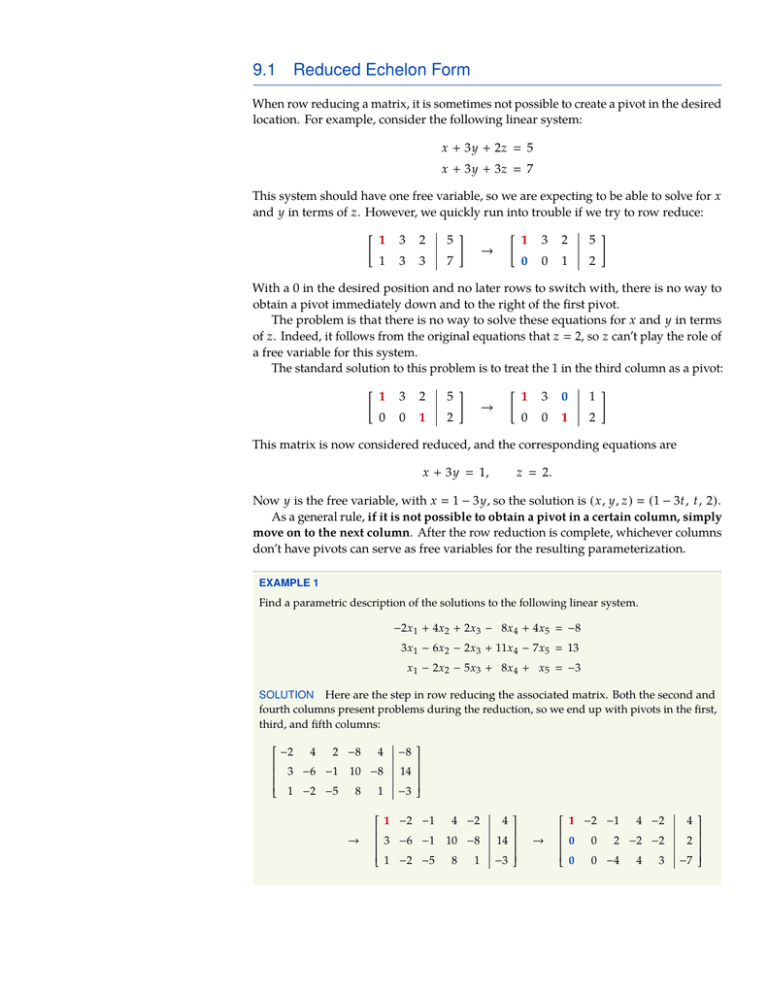
9.1
Reduced Echelon Form
When row reducing a matrix, it is sometimes not possible to create a pivot in the desired
location. For example, consider the following linear system:
x + 3y + 2z 5
x + 3y + 3z 7
This system should have one free variable, so we are expecting to be able to solve for x
and y in terms of z. However, we quickly run into trouble if we try to row reduce:
"
1
3
1
3
2
5
#
"
→
3
7
1
3
2
5
0
0
1
2
#
With a 0 in the desired position and no later rows to switch with, there is no way to
obtain a pivot immediately down and to the right of the first pivot.
The problem is that there is no way to solve these equations for x and y in terms
of z. Indeed, it follows from the original equations that z 2, so z can’t play the role of
a free variable for this system.
The standard solution to this problem is to treat the 1 in the third column as a pivot:
"
1
3
0
0
2
5
#
"
→
1
2
1
3
0
1
0
0
1
2
#
This matrix is now considered reduced, and the corresponding equations are
x + 3y 1,
z 2.
Now y is the free variable, with x 1 − 3y, so the solution is ( x, y, z ) (1 − 3t, t, 2) .
As a general rule, if it is not possible to obtain a pivot in a certain column, simply
move on to the next column. After the row reduction is complete, whichever columns
don’t have pivots can serve as free variables for the resulting parameterization.
EXAMPLE 1
Find a parametric description of the solutions to the following linear system.
−2x 1 + 4x2 + 2x3 − 8x4 + 4x5 −8
3x1 − 6x 2 − 2x3 + 11x4 − 7x5 13
x1 − 2x 2 − 5x3 + 8x4 + x5 −3
SOLUTION
Here are the step in row reducing the associated matrix. Both the second and
fourth columns present problems during the reduction, so we end up with pivots in the first,
third, and fifth columns:
 −2 4 2 −8 4

 3 −6 −1 10 −8

 1 −2 −5 8 1
→
−8 


−3 
14 
 1 −2 −1 4 −2

 3 −6 −1 10 −8

 1 −2 −5 8 1
4 

14 

−3 
→
 1 −2 −1 4 −2

 0 0 2 −2 −2

 0 0 −4 4 3
4 


−7 
2 
REDUCED ECHELON FORM
2
 1 −2 −1 4 −2

 0 0 1 −1 −1

 0 0 −4 4 3
→
→
4 

1 

−7 
 1 −2

 0 0

 0 0
→
 1 −2

 0 0

 0 0
3 −3
5 
1 −1 −1

1 

3 
0
0
0
1
3 −3
5 
1 −1 −1


−3 
0
0 −1
0
→
 1 −2

 0 0

 0 0
1 
3
0
14 
1 −1
0
4 
0
1
0
0


3 
The free variables are x2 and x4 , since these are the columns without pivots, and we have the
equations
x1 − 2x 2 + 3x4 14,
x3 − x4 4,
x5 3.
Thus the solution is
x1 14 + 2s − 3t,
x 2 s,
x3 4 + t,
x4 t,
x5 3.
Reduced Matrices
A matrix that has been reduced through row reduction is said to be in reduced echelon
form. The word echelon is a military term that refers to certain diagonal formations
of troops, ships, or aircraft. For a matrix in reduced echelon form, the pivots form a
diagonal “echelon” across the matrix.
Reduced Echelon Form
A matrix is in reduced echelon form if it satisfies the following conditions:
a U.S. Navy aircraft flying in an echelon
formation.
1. The first nonzero entry in each row is a 1. These 1’s are called pivots.
2. All other entries in the same column as a pivot are zeroes.
3. The pivot in each row lies to the right of the pivot in the previous row.
4. Any rows of zeroes are at the bottom of the matrix.
Here are some of the possible shapes for a matrix in reduced echelon form. Each ∗
represents an arbitrary real number.
 1

 0
 0

 0
"
0
∗ 
1

∗ 

0
0 
0

0 

 1

 0

 0
0
 1

 0

 0
1
0
∗
∗
∗
0
1
∗
∗
∗
∗ 
0
1
0
0
1
0
∗
0 
1
∗
0
0

0 

1 
#
 1

 0

 0

∗ 

∗ 
"
∗
∗ 
1
∗
0
0

∗ 

0 
1
∗
0
 0

 0

 0
0
0
0
0
1
∗
0
∗
∗
0
0
1
∗
∗
#
 1

 0

 0
0 

1 

0 
"
∗
0
∗ 
0
1
0
0


0 
∗ 
 0

 0

 0
1
0
∗ 
0
1
0
0


0 
0
0
1
∗
0
0
0
0
0
1
∗ 
#
REDUCED ECHELON FORM






1
∗
∗
0
∗ 

∗ 

0 

0 
0
0
0
1
0
0
0
0
0
0
0
0
3






1
∗
∗
0
0 

0 

1 

0 
0
0
0
1
0
0
0
0
0
0
0
0






1
∗
0
∗
∗
0
0
0
1
∗
∗
0
0
0
0
0
0
1
0
0
0
0
0
0
∗ 


∗ 

0 
∗ 
A matrix that is in reduced echelon form is called a reduced echelon matrix.
Uniqueness of the Reduced Matrix
As we have seen, it is always possible to use elementary row operations to put a matrix
into reduced echelon form using the Gauss-Jordan elimination algorithm. At this
point we have learned the full algorithm, which is shown in Figure 1.
Two matrices are called row equivalent if it it possible to go from the first matrix to
the second by a sequence of row operations. Using Gauss-Jordan elimination, we can
show that any matrix is row equivalent to a reduced echelon matrix. In fact, a stronger
statement is true.
Uniqueness of the Reduced Echelon Form
Every matrix is row equivalent to a uniquely determined reduced echelon matrix.
That is, if we use any sequence of elementary row operations to put a matrix
d
Figure 1: The full Gauss-Jordan
elimination algorithm for a nonzero matrix.
REDUCED ECHELON FORM
4
into reduced echelon form, we get the same result that we would by performing
Gauss-Jordan elimination. Indeed, there are many matrices for which Gauss-Jordan
elimination is not the simplest route to reducing the matrix.
EXAMPLE 2
Row reduce the following matrix.
3 
 7 15

 2 4


2 
SOLUTION
Using the Gauss-Jordan method, the “proper” first step would be to multiply the
first row by 1/7 to create a pivot. However, this leads to a huge mess of fractions:
 7 15

 2 4
3 

2 

 1 15/7

 2 4
→
3/7 
→

2 

 1 15/7

 0 −2/7
 1 15/7

 0 1
→
3/7 


8/7 
3/7 

−4 

 1

 0
0
→
9 
1
−4 
 1

 0
0
→
9 
1
−4 


A better approach is to start by switching the two rows:
 7 15

 2 4
3 

2 

 2 4

 7 15
→
→
 1 2

 7 15
2 


3 
1 
→

3 

 1

 0
2
1 
1

−4 



We get the same reduced echelon form either way, but the second computation is much easier.
EXAMPLE 3
Row reduce the following matrix.
 5 −2

 2 −1
1 

−1 
SOLUTION
Again, the Gauss-Jordan method tells us that we should multiply the top row
by 1/5. But it works much better to add −2 times the second row to the first row:
 5 −2

 2 −1
1 

−1 
→
 1 0

 2 −1
3 

−1 
→
 1 0

 0 −1
3 

−7 
→
 1

 0
0
3 
1
7 

REDUCED ECHELON FORM
5
A Closer Look Partial Pivoting
Here 1e−20 denotes 1 × 10−20 , i.e. the
number
0.000 000 000 000 000 000 01
Although Gauss-Jordan elimination works well for hand computations, certain modifications
are required for implementing numerical row reduction on a computer. For example, the
matrix
 1e−20 1 1
2 


1 0
0 
 −1

 −1
0 
0 1
should give a solution very close to ( x, y, z ) (1, 1, 1) , but row reducing this matrix on a
computer using Gauss-Jordan elimination can lead to disaster:
 1e−20 1

1
 −1
 −1
0
When using floating point numbers, the
sum of 1e20 and 1 is automatically
rounded to 1e20.
1
2 
0

0 

0 
1
→
 1 1e20 1e20 2e20 


1
0
0 
 −1

 −1
0 
0
1
→
For example, double-precision (72-bit)
floating-point numbers usually keep
track of 60 binary digits, which is about
the same as 18 decimal digits.
→
 1 1e20 1e20 2e20 


1
1
2 
 0
 0 1e20 1e20 2e20 
→
 1

 0
 0
0
0
0 
1
1
2 
0
0


0 
The problem is that computers use floating-point numbers, which only keep track of a certain
number of significant digits. In the second step, the sum of 1e20 and 1 was automatically
rounded to 1e20 in both the second and third rows, leading to a significant loss of information.
This effect can be mitigated using a technique called partial pivoting. In partial pivoting,
we always use the largest entry available in a column to make a pivot. Thus, we would start by
switching the first row with one of the later rows:
 1e−20 1

1
 −1
 −1
0
1
2 
0

0 

0 
1
→
→
The question of how to perform
numerical computations quickly and
accurately on a computer is central to the
fields of scientific computing and
numerical analysis.
 1 1e20 1e20 2e20 


 0 1e20 1e20 2e20 
 0 1e20 1e20 2e20 
 −1
1

 1e−20 1
 −1
0
 1 −1

 0 1
 0 −1
0
0 
1

2 

0 
1
0
0 
1

2 

0 
1
 1
−1

 1e−20 1
 −1
0
→
→
···
→
0
0 
1
2 


0 
1
 1

 0
 0
0
0
1 
1
0
1 
0
1


1 
Partial pivoting is just one of many techniques that mathematicians and computer scientists
have developed to minimize roundoff error during row reductions and other mathematical
computations.
EXERCISES
1–4
Find a parametric description of the solution set for the linear system that
corresponds to the given matrix.
 1

1.  0

 0
3
0
2
5
0
0
1
4
0
0
0
0
0
0
1
0 

2 

6 
 0

2.  0

 0
1
2
0
5
3 
0
0
1
1
4 
0
0
0
0


0 
REDUCED ECHELON FORM
"
−1
3.
2 −1
4
−2
2 −8 −7 −4
 1

5.  2

 1
6
#
7
4
1
1
2
1
0 
8
2
2
4
3
2 
4
1
2
4
3
 1

4.  2

 3
2
2
3
1 
4
4
6
2 
6
6
7


2 


1 
6. Find a 2 × 4 linear system whose solution set can be described parametrically as
( x1 , x2 , x3 , x4 ) (2 − s + 3t, s, 1 − 4t, t )
7–10
State the next elementary row operation that would be used to reduce the
given matrix according to the Gauss-Jordan elimination algorithm.
 1

7.  0

 0
5
 0

9.  0

 1
0
2
5
0
1
2
0
0
0
0
3
0
0
2
6
0
1
3
2
0
0
0
3
7 

1 

9 
4 

7 

9 
 1

8.  0

 0
3
7
8
5
4 
0
0
1
4
2 
0
2
8
4
 1

10.  0

 0
3
5
2
5
4 
0
0
1
5
2 
0
0
0
3


8 


6 
Reduce the given matrix to reduced echelon form using any elementary row
11–16
operations that you like. (You should be able to avoid using fractions.)
"
−4 −7
2
#
"
11.
5
3
7
4
4
3
5
2
#
12.
5
"
5
5
7
6
11
9
2
−3
13.
 7 −8 −8

3
0
15.  −3

 8 −8 −9
#
"
14.
25 

−6 

25 
7 −6
−9
7 −4
1
 2

16.  3

 4
#
4
5
4 
6
2
−5 
8
3


−6 
9.2
The philosophy of mathematics is the
branch of philosophy that considers the
reality of mathematical objects and the
nature of mathematical truth.
As with most statements in philosophy,
the assertions being made here are hardly
noncontroversial. For example, a
mathematical platonist, who believes in
the independent reality of mathematical
objects, would reject the notion that R4 is
any less of a geometric space than the
world that we live in.
Higher Dimensions
It is time for us to tackle the idea of n-dimensional space a little more directly. Here
n-dimensional space refers to a geometric space Rn with n spatial dimensions, where
n can be any positive integer. For example, R1 is an infinite line, R2 is an infinite plane,
and R3 is a three-dimensional space that is infinite in all directions. When n ≥ 4, the
space Rn is said to be higher-dimensional.
Before we discuss the mathematics of higher-dimensional spaces, a few words about
philosophy are in order. There is a basic philosophical objection to higher-dimensional
spaces, which is that there are only three dimensions in the physical world. What does
it even mean to discuss the geometry of four or five-dimensional space if these spaces
don’t really exist?
The answer is that we don’t need these spaces to exist physically to be able
to talk about them. Four and five-dimensional spaces exist on the same level as
other mathematical objects, such as the number 10, the function f ( x ) x 2 , or the
interval [−1, 1]. None of these things have any real physical existence—they are
abstractions, which exist in the sense that they refer to certain aspects of real things.
Thus we can have ten books, or the temperature can be ten degrees, but the number 10
itself isn’t real in any physical sense.
What four-dimensional space refers to is the set of possibilities for a system that
can be described by four real variables. For example, if a chemical reaction involves
four different reactants, then the concentrations ( C 1 , C2 , C 3 , C 4 ) of the reactants are an
ordered quadruple of real numbers. If a sector of the economy involves four goods,
then the prices ( p1 , p2 , p 3 , p4 ) of the goods are an ordered quadruple of real numbers.
In each case, the set of all possible values for this quadruple can be thought of as a
four-dimensional space, with each specific quadruple being a point in this space.
The reason we refer to Rn as a “space” is that we would like to extend our geometric
intuition for R2 and R3 to higher dimensions as much as possible. It turns out that
Rn is similar enough to R2 and R3 that it helps to think about it in geometric terms.
But when we refer to a quadruple such as (5, 3, 2, 7) as a “point” in R4 , we are really
just making an analogy to points in R2 and R3 . Because higher-dimensional spaces
only exist in the abstract, we must always be very careful to define geometric terms
precisely before using them in this context. For example, the term “distance” seems
self-explanatory in two and three dimensions, but for higher dimensions we must say
exactly what we mean by “distance” before we can use this concept.
Thus, our description of higher dimensions will include precise definitions of
many basic geometric concepts. In most cases, these definitions will be based on
the descriptions of these concepts that we obtained in R2 and R3 . For example,
the Pythagorean theorem is a theorem of Euclidean plane geometry, but in higher
dimensions it becomes part of the definition of distance.
Vectors in Rn
A vector (or point) in n dimensions is simply a list of n real numbers. We can write a
vector as either a tuple or as a column vector.
The ellipses (· · ·) in this equation
represent the components of v numbered
between v2 and v n .
 v1 
 
 v2 
v ( v 1 , v2 , . . . , v n )  . 
 .. 
 v n 
HIGHER DIMENSIONS
2
The numbers v1 , v2 , . . . , v n in the list are called the components of the vector v. The set
of all such vectors with n components is denoted Rn , and is referred to as n-dimensional
Euclidean space or simply n-dimensional space.
In R2 and R3 , we defined addition of vectors geometrically using arrows, and then
worked out that it corresponds to the componentwise sum. For higher dimensions,
though, we use componentwise sum as the definition of addition.
 v1 
 w1 
 v1 + w1 
 




 v2  +  w2   v2 + w2 
..
 ... 
 ... 


.
 




 vn 
 wn 
 v n + w n 
a Figure 1: The sum of two vectors in R
can be thought of geometrically using
arrows.
n
We imagine vector addition as having the same geometric meaning in higher dimensions
that it does in R2 and R3 , as shown in Figure 1.
Scalar multiplication is defined componentwise:
 v1 
 kv1 
 


v2 
kv2 





k  .   . 
 .. 
 .. 
 v n 
 kv n 
Again, we imagine this as having the same geometric meaning that it does in R2 and R3 .
That is kv is a vector in the same direction as v (if k > 0) or in the opposite direction
as v (if k < 0), but whose length has been scaled by a factor of |k|.
If v1 , v2 , . . . , vk are vectors in Rn , a linear combination of v1 , v2 , . . . , vk is any vector
of the form
c1 v1 + c2 v2 + · · · + c k vk
where c 1 , c 2 , . . . , c k are scalars.
EXAMPLE 1
Express the vector (4, 5, 10, 1) as a linear combination of the vectors (1, −1, 1, 1) , (−1, 4, 1, −2) ,
and (2, 10, 10, −2) .
SOLUTION
We wish to find scalars c1 , c2 , and c3 so that
 1 
 −1 
 2 
 4 






 
−1
4
10
 + c2 
 + c3 
  5 
c 1 
 1 
 1 
 10 
 10 
 1 
 −2 
 −2 
 1 
The vector equation is equivalent to a linear system with 4 equations a 3 unknowns, which we
can solve using row reduction.
 1 −1 2

 −1 4 10

 1 1 10
 1 −2 −2
 1 −1 2


0
3 12
5 
 → 
 0 2 8
10 


1 
 0 −1 −4
4 
 1 −1 2


0
1
4
9 
 → 
 0 2 8
6 


−3 
 0 −1 −4
4 
 1


0
3 
 → 
 0
6 


−3 
 0
4 
0
6
7 
1
4
3 
0
0
0
0


0 

0 
Apparently there are infinitely many different solutions for c1 , c2 , and c3 . Indeed, the first two
rows in the reduced echelon form represent the equation
c1 + 6c 3 7
and
c2 + 4c3 3
HIGHER DIMENSIONS
When only one solution to a linear system
is needed, values for the free variables
can be chosen arbitrarily.
3
so c 3 is a free variable. We only need one solution, so we can pick the value for c 3 and then
solve for c1 and c2 . The easiest choice is c3 0, in which case c1 7 and c2 3. Thus
 1 
 −1 
 2 
 4 






 
−1 
4
10 
5
7 
+ 3 
+ 0 
 



 1 
 1 
 10 
 10 
 1 
 −2 
 −2 
 1 
Incidentally, in the last example, the reason that there were infinitely many solutions
for c 1 , c2 , and c 3 is that the third vector was actually a linear combination of the first
two:
 2 
 1 
 −1 






 10  6  −1  + 4  4 
 10 
 1 
 1 
 −2 
 1 
 −2 
In general, a set of vectors is said to be linearly independent if none of them can be
expressed as a linear combination of the others. For a linearly independent set of vectors,
the coefficients in any linear combination of the vectors are uniquely determined.
Distances and Angles
If v is a vector in Rn , the magnitude of v is the scalar
|v| q
v1 2 + v2 2 + · · · + v n 2
If we imagine v as an arrow in Rn , then |v| can be thought of as the length of this vector.
If we imagine v as a point in Rn , then |v| can be thought of as the distance from this
point to the origin 0 (0, 0, . . . , 0) .
More generally, the distance from a point p to a point q in Rn is defined to be the
magnitude of the difference p − q, i.e.
|p − q| q
( p1 − q1 ) 2 + ( p2 − q2 ) 2 + · · · + ( p n − q n ) 2
The dot product of two vectors v, w in Rn is defined by
v · w v1 w1 + v2 w2 + · · · + v n w n
We say that v and w in Rn are orthogonal if v · w 0. We imagine orthogonal vectors
as pointing at right angles in Rn .
More generally, we can use the dot product to define the angle between two vectors.
Specifically, if v and w are vectors in Rn , the angle θ between them is defined by the
formula
v·w
θ cos−1
|v| |w|
Hyperplanes
The vector ( a 1 , a 2 , . . . , a n ) of coefficients
is the normal vector to the hyperplane.
As mentioned previously, a hyperplane in Rn is the set defined by a linear equation of
the form
a1 x1 + a2 x2 + · · · + a n x n b
where the coefficients a1 , a2 , . . . , a n are not all zero. We can imagine a hyperplane as
being similar to a line in R2 or a plane in R3 , except that it is an (n − 1)-dimensional set
HIGHER DIMENSIONS
4
in n-dimensional space. A k × n linear system corresponds to k different hyperplanes
in Rn , with the solution set being the intersection of these hyperplanes.
EXAMPLE 2
Find a point in R4 that lies on both of the following hyperplanes.
3x1 + 6x2 + 5x3 + 2x4 5
We make the two equations into a linear system and row reduce.
SOLUTION
In the first step of this row reduction we
subtract the second row from the first.
This avoids the fractions that would result
from multiplying the first row by 1/3.
 3

 2
6
4
2x1 + 4x2 + 3x 3 + 7x4 8
5
3
2
5 
7

8 
 1

 2
→
 1

 0
→
2 −5
2
0
→
7

8 
−5
−3 
1 −17

−14 
4
2
−3 
3
2
→
 1

 0
 1

 0
2 −5
−3 
0 −1 17
14 
2

2
0
29
25 
0
1 −17
−14 

This gives the equations
x1 + 2x2 + 29x4 25
Another possibility would be x2 0 and
x4 1, which gives the point (−4, 0, 3, 1) .
and
x3 − 17x4 −14
where x2 and x4 are free variables. We only want one point, so we can pick any values for x 2
and x4 and then solve for x1 and x3 . One possible choice is x2 x4 0, in which case x 1 25
and x3 −14. Thus (25, 0, −14, 0) is a point that lies on both hyperplanes.
We can also use row reduction to find an equation for a hyperplane that goes
through a given set of a points. This
EXAMPLE 3
Find an equation for any hyperplane in R4 that goes through the points (1, 2, 3, 1) and (3, 7, 4, 3) .
SOLUTION
The desired equation has the form
a1 x1 + a2 x2 + a3 x3 + a4 x4 b
Substituting in the two points gives a 2 × 5 linear system with a1 , a2 , a3 , a4 , and b as unknowns.
a1 + 2a2 + 3a3 + a 4 − b 0
Note that we moved the b’s to the left side.
3a1 + 7a2 + 4a3 + 3a 4 − b 0
We row reduce the corresponding matrix.
 1 2 3 1 −1

 3 7 4 3 −1
0 

0 

→
 1 2 3 1 −1

 0 1 −5 0 2
0 

0 

→
 1 0 13 1 −5

 0 1 −5 0 2
0 


0 
This gives the equations
a1 + 13a3 + a4 − 5b 0
and
a2 − 5a3 + 2b 0
where a3 , a4 , and b are free variables. We can pick any values for these variables except for
a3 a4 b 0, since this would lead to all the coefficients being zero. We choose a 3 a 4 0
and b 1, which gives a1 5 and a2 −2. Thus, one hyperplane that contains the given
points is
5x1 − 2x2 1
HIGHER DIMENSIONS
5
EXERCISES
1. Find the distance between the points (5, 1, 3, 7, 6) and (4, 2, 6, 9, 5) in R5 .
 1 
 5 
 


2
−1 
2. Find the angle between the vectors   and 
in R4 .
 3 
 5 
 4 
 3 
Express the vector w as a linear combination of u and v, or state that this is not
possible.
3–4
 −2 
 3 


3. u  1  , v  −1 


 −3 
 −4 
 5 


 4  , w  −2 
 −7 
 8 
 −15 


 2 
 4 
 9 
 2 


−1 
4. u 
, v
 −3 
 −2 
 2 


 −4  , w  −5 
 −3 
 4 


 1 
 −4 
 −1 
5. Find any point in R3 that lies on both the plane 2x − 8y − 2z −4 and the plane
x − 2y + 3z −8.
6. Find the equation for any hyperplane in R4 that contains the points (1, 2, 1, 3) ,
(2, 5, 3, 1) , and (7, 16, 7, 5)
7. Find any nonzero vector in R4 that is orthogonal to each of the three vectors
(1, 4, 0, 4) , (2, 7, 3, 10) , and (3, 10, 8, 20) .