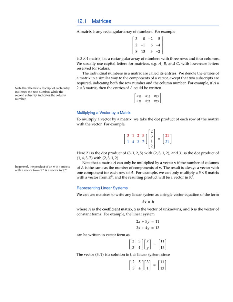
12.1
Matrices
A matrix is any rectangular array of numbers. For example
 3 0 −2 5 


 2 −1 6 −4 


 8 13 3 −2 
Note that the first subscript of each entry
indicates the row number, while the
second subscript indicates the column
number.
is 3 × 4 matrix, i.e. a rectangular array of numbers with three rows and four columns.
We usually use capital letters for matrices, e.g. A, B, and C, with lowercase letters
reserved for scalars.
The individual numbers in a matrix are called its entries. We denote the entries of
a matrix in a similar way to the components of a vector, except that two subscripts are
required, indicating both the row number and the column number. For example, if A a
2 × 3 matrix, then the entries of A could be written
"
a11
a21
a12
a22
a 13
a 23
#
Multiplying a Vector by a Matrix
To multiply a vector by a matrix, we take the dot product of each row of the matrix
with the vector. For example,
 
#  2 
"
#
21
 3 
 
1 4 3 7  1 
31
 2 
Here 21 is the dot product of (3, 1, 2, 5) with (2, 3, 1, 2) , and 31 is the dot product of
(1, 4, 3, 7) with (2, 3, 1, 2) .
"
In general, the product of an m × n matrix
with a vector from Rn is a vector in Rm .
3 1 2 5
Note that a matrix A can only be multiplied by a vector v if the number of columns
of A is the same as the number of components of v. The result is always a vector with
one component for each row of A. For example, we can only multiply a 5 × 8 matrix
with a vector from R8 , and the resulting product will be a vector in R5 .
Representing Linear Systems
We can use matrices to write any linear system as a single vector equation of the form
Ax b
where A is the coefficient matrix, x is the vector of unknowns, and b is the vector of
constant terms. For example, the linear system
2x + 5y 11
3x + 4y 13
can be written in vector form as
"
2
5
3
4
x
#" #
y
"
11
#
13
The vector (3, 1) is a solution to this linear system, since
"
2
5
#" #
3
3
4
1
"
11
13
#
MATRICES
2
Matrix Multiplication
There is an operation called matrix multiplication that generalizes the product of a
matrix and a vector. Given two matrices A and B, the product AB is the matrix obtained
by taking the dot product of each row of A with each column of B. For example, if A
and B are 2 × 2 matrices, then there are four dot products to compute:
"
"
If A is an m × n matrix, and B is an n × p
matrix, then AB is an m × p matrix.
7
5
1
2
#"
7
5
1
2
#"
2
0
3
1
#
2
0
3
1
#
"
"
#
14
14
10
22
#
"
"
7
5
1
2
#"
7
5
1
2
#"
2
0
3
1
#
2
0
3
1
#
"
14
22
#
"
14 22
10 17
#
This product only makes sense if the rows of A and the columns of B are vectors of
the same size. In the example above, the rows of A and the columns of B are vectors
from R2 , which makes it possible to take the dot products. In general, the matrix
product AB is only defined if the number of columns of A is equal to the number of
rows of B.
When we compute the product AB, the result always has one row for each row of A
and one column for each column of B. For example, if A is a 3 × 5 matrix and B is a
5 × 7 matrix, then AB is a 3 × 7 matrix.
EXAMPLE 1
 7

Compute AB if A  3
 1
5
1
6
2
1
3
 0
2 

2

0  and B 

 2
0
 1
3 

2 
.
4 

0
SOLUTION Since A has three rows and B has two columns, the product AB is a 3 × 2 matrix.
To compute the entries of this matrix, we must take the dot product of each row of A with
each column of B.
 7
 3

1
5
1
6
2
1
3
0
2  
2
0  
2
0  
1
3  
16

2  

4  

0  
 7
 3

1
5
1
6
2
1
3
0
2  
2
0  
2
0  
1
3  
16

2  
 4

4 

0  
 7
 3

1
5
1
6
2
1
3
0
2  
2
0  
2
0  
1
3  
16

2  

4
4  
  18
0




 7
 3

1
5
1
6
2
1
3
0
2  
2
0  
2
0  
1
3  
16

2  

4  

0  
39 
 7
 3

1
5
1
6
2
1
3
0
2  
2
0  
2
0  
1
3  
16

2  
 4

4 

0  
 7
 3

1
5
1
6
2
1
3
0
2  
2
0  
2
0  
1
3  
16

2  

4
4  
  18
0



39 

15 


39 



39 

15 


39 

15 

27 
Note that the product of a matrix A and a vector v is actually a special case of matrix
multiplication. In particular, if we think of a vector v from Rn as a matrix with one
column (i.e. an n × 1 matrix), then Av is the same as the product of the matrices A
and v.
MATRICES
3
Properties of Matrix Multiplication
If A is an m × n matrix and B is an n × m matrix, then we can multiply them in either
order, giving us two different products AB and BA. Surprisingly, these products are
not usually the same! For example, if A is a 3 × 5 matrix and B is a 5 × 3 matrix, then AB
is a 3 × 3 matrix and BA is a 5 × 5 matrix, so AB and BA do not even have the same size!
Even if AB and BA have the same size, they are usually not the same matrix. For
example,
"
3
2
#"
1
2
7
1
1
2
#
"
22
16
5
6
#
"
and
7
1
1
2
#"
3
2
1
2
#
"
23 9
7 4
#
In the language of abstract algebra, matrix multiplication is not a commutative operation.
Though matrix multiplication is not commutative, it is associative. That is, if A, B
and C are matrices, then
A ( BC ) ( AB ) C
Thus we can unambiguously write a product like ABC, without specifying whether A
and B should be multiplied first or B and C should be multiplied first.
For each n, there is a special n × n matrix called the identity matrix, which is usually
denoted by the letter I. The 2 × 2, 3 × 3, and 4 × 4 identity matrices are shown below.
"
The identity matrix I can be thought of as
a matrix analog of the number 1.
1
0
0
1
 1

 0
 0
 0
 1 0 0 
 0 1 0 


 0 0 1 
#
0
1
0
0
0
0
1
0
0 

0 
0 

1 
The identity matrix has the special property that AI A whenever AI is defined, and
IB B whenever IB is defined. For example,
"
1
0
0
1
#"
2
6
5
9
2
9
#
"
2
6
5
9
2
9
 2 3  "
2 3
#
 1 4  1 0  1 4 

 0 1


 1 5 
 1 5 
#
and
Addition and Scalar Multiplication
Matrix subtraction is defined in a similar
way.
There are three more basic operations involving matrices: addition, scalar multiplication,
and transpose. Matrix addition works just like vector addition, with corresponding
entries of the two matrices added together:
"
2
2
1
1
1
5
#
"
+
3
5
5
2
1
2
#
"
5
7
6
3
2
7
#
Only two matrices of the same size can be added. Matrix multiplication distributes
over addition from both the left and the right, i.e.
A ( B + C ) AB + AC
and
(A + B ) C AC + BC
Scalar multiplication for matrices is also quite similar to scalar multiplication for
vectors:
"
#
"
#
4 3 1
8 6 2
2
4 2 3
8 4 6
This has a variety of obvious properties, e.g.
k ( A + B ) kA + kB
for any scalar k and matrices A and B.
and
k ( AB ) ( kA ) B A ( kB )
MATRICES
4
Matrix Transpose
The transpose of a matrix is obtained by switching its rows with its columns. For
example, the matrices
 1 0 
"
#
1 5 3
 5 2 
and


0 2 4
 3 4 
are transposes of one another. If A is a matrix, its transpose is usually denoted AT .
Taking the transpose reverses the order of matrix multiplication. That is,
(AB ) T B T AT
for any matrices A and B. For example,
"
1
0
5
2
3
4
#  1 4 
"
#
 3 1  22 18


14 14
 2 3 
"
and
1
4
3
1
2
3
#  1 0 
"
#
 5 2  22 14


18 14
 3 4 
Note also that the transpose of a transpose is the original matrix, i.e.
AT
T
A
Special Kinds of Matrices
A square matrix is a matrix with the same number of rows and columns, such as a
2 × 2 matrix, a 3 × 3 matrix, or more generally an n × n matrix. We can multiply any two
square matrices of the same size, with the product being another matrix of that size.
A square matrix is symmetric if it is equal to its own transpose. For example,
"
It is all right if some of the diagonal
entries of a diagonal matrix are zero. For
example,
3 0
0 0
is a perfectly good diagonal matrix.
2
4
4
3
#
and
 3 5 1 
 5 9 6 


 1 6 4 
are symmetric matrices. Note that the diagonal entries of a symmetric matrix (highlighted in red) can be any numbers at all, but the off-diagonal entries must be equal in
pairs.
A diagonal matrix is a square matrix whose off-diagonal entries are all zero. For
example,
 5 0 0 
"
#
4 0
 0 2 0 
and


0 3
 0 0 6 
are diagonal matrices. Note that a diagonal matrix is always symmetric. Diagonal
matrices are particular easy to multiply: one need only multiply the corresponding
diagonal entries. For example,
 1 0 0   5 0 0 
5 0 0 
 0 2 0   0 7 0   0 14 0 





 0 0 3   0 0 11 
 0 0 33 
An upper-triangular matrix is a square matrix that has zeroes below the main
diagonal. For example,
"
4
0
2
3
#
and
 5 3 1 
 0 2 7 


 0 0 6 
MATRICES
5
are upper-triangular. The product of two upper-triangular matrices of the same size is
again upper-triangular, e.g.
"
3
0
2
4
#"
2
0
#
2
1
"
6
0
8
4
#
Note that every diagonal matrix is upper triangular, and that a matrix is diagonal if
and only if it is both upper-triangular and symmetric.
The transpose of an upper-triangular matrix is called a lower-triangular matrix.
Such matrices have zeroes above the main diagonal:
"
4
2
0
3
 5 0 0 
 3 2 0 


 1 7 6 
#
and
Again, the product of two lower-triangular matrices is lower-triangular. Note that a
matrix is diagonal if and only if it is both upper triangular and lower triangular.
EXERCISES
 8 0 4 6 


1. If A  3 1 2 4  , what is a 23 ?


 5 7 5 1 
Multiply.
2–5
 −9

2.  2

 3
 1

2
4. 
 0
 6
 −5

1
3. 
 9
 −1
3
1   −3 


9 −3   1 
 

0
8   1 
7
8
1
9
2
2
1
2
2   0 
 
1   1 
2   0 
 
2   0 
 0

0
5. 
 0
 0
1
6
5
1
0   
 4
0   
0
3   
  2 
0
Find a vector x such that Ax b.
6–7
"
−8
6. A 1
#
"
9
−20
, b
−3
10
#
8. Find the values of x and y for which
"
9.
"
 6 4
2 


7. A  1 2 −2  , b 

 1 1 −3 
"
#" # " #
x
4
1
−2
y
2
 2 
 5 
 
7
8
.
0
Multiply.
9–14
11.
1  "
#

7  5
0  −2

1 
6
4
3
−1
#"
1
0
3
−8
#"
−1
8
1
3
2
1
3
0
#
"
1
9
f
1
10.
2
2
#
12.


#  −1 −4 
3
9
1  0 −1 
2 
1 −2 −2  2


0 
 −6
g " 3 −4 #
7
1
−1
MATRICES
13.
f
8
6
−1


g  2 
7  3


 −1 
14.
" #f
2
3
3 −2
1
g
15. Let A and B be 3 × 3 matrices, and let C AB. Given that
a32 b32 0,
a31 4,
b12 3,
and
what is the value of c32 ?
"
0
16. If A 2
#
1
, compute ATA − 3A.
3
" #
"
#
2
8
17. Find a 2 × 2 diagonal matrix A such that A
.
3
−6
"
18. Find a 2 × 2 upper-triangular matrix A such that A + AT "
19. Find a 2 × 2 matrix A such that 4A −
2AT
6
2
#
6
5
5
.
8
#
8
.
2
20. Find a 2 × 2 symmetric matrix A such that
" #
" #
1
A
0
5
3
and
f
0
g
1 A
f
3
g
4 .