A residual from updating based approach for
multiple categorical ordinal responses
Giulio D’Epifanio1
Department of Economy, Finance and Statistics, University of Perugia, via A.
Pascoli, 06100 Perugia, Italy, giulio@stat.unipg.it
Summary. To analyze multiple categorical ordinal responses, a pseudo-Bayes approach is proposed which uses estimating equations based on the Constrained Fixed
Point methodology.
Key words: constrained fixed point, multiple categorical ordinal data, pseudoBayes
1 Introduction
In social inquires about perceived health, a typical questionnaire contains queries as the following: How do you consider your
health status? Thus, ordinal responses as the following Y quest. ∈
{”V ery bad”, ”Bad”, ”M oderate”, ”Good”, ”Excellent”} are typically considered
over a L-point (L := 5) verbal descriptor scale. Focusing interest in problem
diagnostics, the original categories of Y quest. may be properly re-codified in
those of ”Severity” Y ∈ {N one, M ild, M oderate, Severe, V ery severe}, so that
higher levels of Y indicate higher level of difficulty.
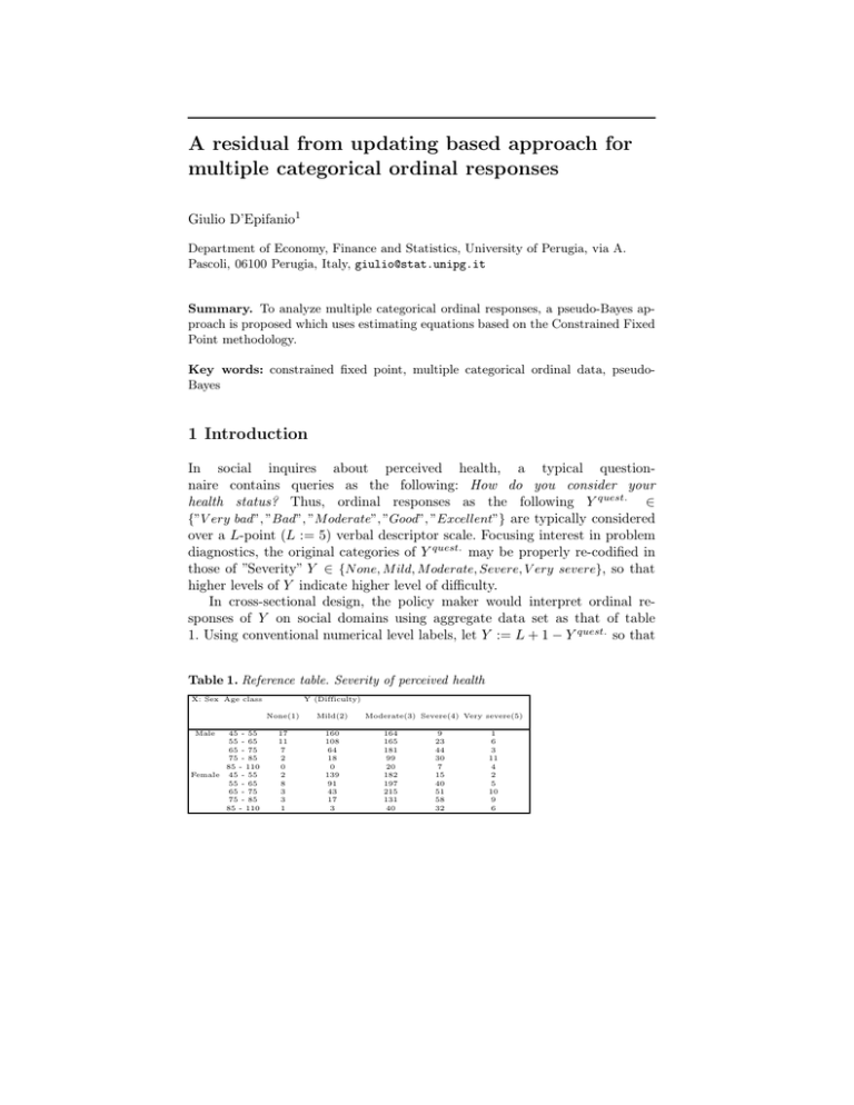
In cross-sectional design, the policy maker would interpret ordinal responses of Y on social domains using aggregate data set as that of table
1. Using conventional numerical level labels, let Y := L + 1 − Y quest. so that
Table 1. Reference table. Severity of perceived health
X: Sex Age class
Male
45 - 55
55 - 65
65 - 75
75 - 85
85 - 110
Female 45 - 55
55 - 65
65 - 75
75 - 85
85 - 110
Y (Difficulty)
None(1)
Mild(2)
17
11
7
2
0
2
8
3
3
1
160
108
64
18
0
139
91
43
17
3
Moderate(3) Severe(4) Very severe(5)
164
165
181
99
20
182
197
215
131
40
9
23
44
30
7
15
40
51
58
32
1
6
3
11
4
2
5
10
9
6
566
Giulio D’Epifanio
Y ∈ {”1”, ”2”, . . . ”L”}. Over the ordinal categories of Y quest. , assume the
choice process for respondents1 which is sketched in figure 1. Thus, reversing Y quest. to Y , the main substantive concern is in detecting latent rules
which govern, for any severity level l := 2, . . . , L of Y , the ”resistance of lower
severity levels against further aggravation up to l”, by considering both social
strata (induced by sex and age) and current level effects.
Fig. 1. Choice process over Y quest. : partitioning of categories
A recursively structured model would be necessary to interpret table 1.
Unfortunately, in the ”constrained multinomial model”(CMM) setup2 , the full
maximum likelihood approach may be difficult to implement.
In a non standard framework, the Prior Feedback Setup has been proposed
(Casella & Robert, 2002, pp. 203-204) which uses pseudo-Bayes tools. In this
type of inferential framework, D’Epifanio proposed (1996) the ”Fixed Point”
(FP) approach and delineated (1999) the ”Constrained Fixed Point” (CFP),
which has been recently (D’Epifanio, 2004) applied to analyze contingency
tables. Briefly, CFP would match ”candidate priors”, which are parametrized
over conjectured belief-model, to ”posterior” attempting to minimize ”residual from updating”. It provides a type of estimating equation which elicits
data dependent prior (Agresti, 1990, pp. 466). Inferences are very close to
that of maximum likelihood (ML) whenever the likelihood function is sufficiently regular. Thus, typical ML-diagnostic tools may be also considered.
But, since CFP is pseudo-Bayes, it could even work better than ML whenever the likelihood function is pathological (Robert et al., 1993; D’Epifanio,
1996) or parameter smoothing is also requested. On the other hand, CFP data
1
Consider the original question Y quest. . Having started (see figure 1) from the
lower (”Very bad”) level sequentially ascending levels, suppose respondent i is temporarily arrived up to level r-th of the scale of Y . Now, he processes the verbal
description at level r-th against descriptions of higher level r + 1, . . . , L. Then, he
passes to the upper-level (r + 1)-th whenever he perceives the added level-specific
requirements Or of satisfaction are met.
2
it provides a framework where usual types (Lunt, 2005) of ordinal models (the
”proportional odds”, the ”continuation ratio”, the ”stereotype model”, etc.) may be
specified
Title Suppressed Due to Excessive Length
567
analysis is insensitive to the risk, which instead is actual in the full bayesian
analysis, of using some misleading specific prior.
Using CFP, powerful numerical procedures may be implemented. In practice, CFP is a machinery which may be useful from both the classical and
Bayesian perspective. For classic statisticians, it could provide advanced starting points for their classical ML based procedures. For Bayesians, it would
provide an operative tool for automatic eliciting of some ”standard” prior,
over preliminary ”reference data set”, to be then used in their bayesian logic.
This work is organized as follows. In section 2, we provide the formal
framework to interpret data table 1, conditional on working conjectures. In
section 3, we recall CFP methodology and provide specific estimating system.
In section 4, we briefly report results of CFP over data table 1.
2 Conceptual framework and statistical modeling
We establish a formal framework to interpret ordinal responses Y of table 1,
conditional on choice process of figure 1 and working conjecture about effects
of both social strata and levels. Model is structured in two main parts: the
”manifest (observation) model” (1) and the underlying ”belief carrier model”
(2-3-4). Working conjectures are depicted3 over the belief carrier model (instead of directly over manifest model (1), see also Agresti et al, 1989), up to
a certain degree of uncertainty which is (in our perception) physiological and
natural in social sciences.
Within the ”belief container” model (2), which is (used as a formal ”blackboard”) a product of Dirichlet’s distributions, the ”belief carrier model” is
hierarchically structured to incorporate assumptions on choice process of figure 1 (eq. 3) and, subsequent nested, on specific working-conjectures about
latent social and level effects (eq. 4) over process.
From observed responses, information will pass through manifest model
(1) to be then interpreted at light of the belief-model (2-3-4).
2.1 The manifest model
ind.
Yi | ψi ∼ M ult(yi ; ψi , ni ), i = 1, . . . , R
(1)
Here, Yi ∈ {yi1 , . . . , yiL } is the (row-)profile (L := 5) which is associated to
the i-th stratum of the R (R := 10) strata of data in table (1). M ult(yi ; ψi , ni )
denotes the multinomial distribution with parameters ψi := (ψi1 , ψi2 , . . . , ψiL ),
where ψil := P r{Yi = ”l”}, l := 1, . . . , L, and size ni .
3
conjectures are structured by constraining the Dirichlet’s distributions in (2) to
have expected values which fulfill specified pattern-conjectures
568
Giulio D’Epifanio
2.2 The belief carrier model
Let Dirich(ψi ; mi , ai ) denote the Dirichlet’s distribution, which is associated
to the stratum i-th, where mi := (mi1 , mi2 . . . , miL ) := E[Ψi ] and ai > 0 is
the usual scalar hyper-parameter4. The belief-carrier model is structured as
follows:
The belief-carrier ”container”:
ind.
Ψi | mi , ai ∼
i:=1,...,R
Dirich(ψi ; mi , ai ),
X
(2)
L
mi := (mi1 , mi2 , . . . , miL ), 0 < mi1 < 1,
mir = 1,
r:=1
ai := wi , wi > 0
Conjecture on the binary choice process (figure 1):
eηi1
mi1
=
,
mi1 + mi2
1 + eηi1
...
mi1 + ... + mi(l−1)
eηi(l−1)
vil :=
=
,
mi1 + mi2 + ... + mil
1 + eηi(l−1)
...
mi1 + ... + mi(L−1)
eηi(L−1)
viL :=
=
,
mi1 + mi2 + ... + mi(L)
1 + eηi(L−1)
(3)
vi2 :=
Working conjecture about latent phenomenon5 which governs choice process:
ηil = µ0 +
L
X
s:=3
Sex
δl I(s=l) + β(l−1)
· I(Sex(i)=”F em.”) +
K
X
r:=2
Age
βr(l−1)
· I(Age(i)=r) ,
(4)
i := 1, . . . , R, l := 2, . . . , L
Let γ := (µ0 , δ, β) denote the full profile of parameters in (4), which are
implicitly interpreted through table 2.
Notes.
• Across strata i := 1, . . . , R, parameter profiles ψi := (ψi1 , ψi2 , . . . , ψiL ) of (1)
are considered as ”virtual” random vectors which are conditionally independent.
The parametric class of product of Dirichlet’s priors provides a convenient coordinate space {(mi , ai ), i := 1, . . . , R} to depict (see sketch in figure 2) working
conjectures as geometric sub-manifolds
m +···+mi(l−1)
is
• Associated to choice process (figure 1), the parameter vil := i1
mi1 +···+mil
interpreted as follows. For social stratum i-th, at current difficulty level l, vil
measures the ”resistance” of lower severity levels against further aggravation up
to level l. Model (4) depicts the conjecture that vil is driven by sex, age, which
are level-specific, and current level l itself.
4
it weights the ”virtual” number of observations that the prior information would
represent (Agresti et al., 1989)
5
in eq. (4), K := 5 denotes the number of category for Age, I(s=l) the indicator function which selects category l-th when s = l, I(Sex=”F em.”) and I(Age=r)
respectively the indicator which selects ”Sex=female” and the r-th age interval.
Title Suppressed Due to Excessive Length
569
Table 2. Interpretation of parameter γ which depicts working conjecture of eq. (4).
Cell (il)-th refers to the effects which govern process parameter vil
X: Sex Age class
Mild (”2”)
Male
45 - 55
55 - 65
65 - 75
75 - 85
85 - 110
Female
45 - 55
55 - 65
65 - 75
µ0
µ0
75 - 85 µ0
85 - 110 µ0
µ0
Age
µ0 + β21
Age
µ0 + β
31
Age
µ0 + β
41
Age
µ0 + β51
Sex
µ0 + β1
Age
Sex
+β
+ β1
21
Age
Sex
+β
+ β1
31
Age
Sex
+ β41
+ β1
Age
Sex
+ β51
+ β1
Moderate (”3”)
µ0
µ0
µ0
µ0
µ0 + δ1
Age
µ0 + δ1 + β22
Age
µ0 + δ1 + β
32
Age
µ0 + δ1 + β
42
Age
µ0 + δ1 + β52
Sex
µ0 + δ1 + β2
Age
Sex
+ δ1 + β
+ β2
22
Age
Sex
+ δ1 + β
+ β2
32
Age
Sex
+ δ1 + β42
+ β2
Age
Sex
+ δ1 + β52
+ β2
Severe (”4”)
µ0
µ0
µ0
µ0
µ0 + δ2
Age
µ0 + δ2 + β23
Age
µ0 + δ2 + β
33
Age
µ0 + δ2 + β
43
Age
µ0 + δ2 + β53
Sex
µ0 + δ2 + β3
Age
Sex
+ δ2 + β
+ β3
23
Age
Sex
+ δ2 + β
+ β3
33
Age
Sex
+ δ2 + β43
+ β3
Age
Sex
+ δ2 + β53
+ β3
Very severe (”5”)
µ0
µ0
µ0
µ0
µ0 + δ3
Age
µ0 + δ3 + β24
Age
µ0 + δ3 + β
34
Age
µ0 + δ3 + β
44
Age
µ0 + δ3 + β54
Sex
µ0 + δ3 + β4
Age
Sex
+ δ3 + β
+ β4
24
Age
Sex
+ δ3 + β
+ β4
34
Age
Sex
+ δ3 + β44
+ β4
Age
Sex
+ δ3 + β54
+ β4
3 The Constrained Fixed Point methodology
3.1 About the CFP setup
The underlying principle of FP, which is of ”least information”, is that (D’Epifanio,
1996) ”the less a candidate prior is updated (that is, the more it would be insensitive
to the Bayesian updating rule if it had actually used as prior), the more it intrinsically already was accounted for by the information added by current data”, conditional
on the assumed model. This leads to a ”what-if” type of criterion. Thus, by formally
interpreting this principle, CFP would search for minimizing the, properly weighted,
”residual from updating”. By formally interpreting this general principle-, we would
minimize” the ”residual from updating”:
k V ec ( E(Ψ | y, x; γ, w) − E(Ψ | x; γ, w) ) k= min .
γ
(5)
Here6 , E(Ψ | y, x; γ, w) is the response-updated predictive expectation given y,
whereas E(Ψ | x; γ, w) is the non response-updated counterpart, of full parameter
profile Ψ , over the design point x. Let ∆T (γ, w) := V ec ( E(Ψ | y, x; γ, w) − E(Ψ |
x; γ, w)).
Of course in model (2), belief-parameters w might be ”a priori” assigned.
But more interesting, they could be determined by actual data to quantify datadependent uncertainty. A further criterion is necessary which is complementary
to that of ”least updating”. Over the coordinate space of belief-carrier manifold (2), we would (D’Epifanio, 1996) the ”virtual information gain” {V ar(Ψ |
x; γ, w) − V ar(Ψ |y, x; γ, w)} meets, the more is possible, with the ”virtual loss”
V ar(Ψ |y; x; γ, w) due to updating induced by response y, given design point x. In
the full FP, there exists a large sample interpretation (D’Epifanio, 1996) of this
principle which is related to the Fisher’s information.
6
For simplicity we consider here belief-parameter w assigned. CFP uses actual
data (table 1) to determine the point-coordinate (see sketch in figure 2) which elicits
(within the proper coordinate space which depicts working model) that potenzial
”candidate prior” such that it ”would be, the more is possible, insensitive to the
bayesian updating if it had actually used as prior”. So it would be conformed, the
more is possible, to the specified (sub-manifold induced by) working conjecture.
570
Giulio D’Epifanio
Fig. 2. CFP: geometrical sketch
Thus, full CFP would search, in proper coordinate space given the design point
x, for that candidate prior which minimizes full residual:
k
V ec ( E(Ψ | y, x; γ, w) − E(Ψ | x; γ, w) )
k= min
V ec V ar(Ψ | y, x; γ, w) − V ec {V ar(Ψ | x; γ, w) − V ar(Ψ | y, x; γ, w)}
γ,w
(6)
Let denote variation here with ∆y;x .
The method is, generally, consistent and efficient. Asymptotics of unrestricted
FP has been delinated in other works (D’Epifanio, 1996, 1999). It is operatively
important to focus attention here on the fact that belief-container model has an
instrumental role in that convergence (D’Epifanio, 1999) to maximum likelihood estimates (under general regularity assumptions when the conjectured depicted model
is adequate) is very fast irrespective of the choice for some specific class of ”candidate
priors”. Thus, without relevant arbitrariness, a criterion may be considered which
uses convenient belief-container models so that updating rules are possibly simple,
easy to implement and computationally efficient.
3.2 Specific CFP formulation for categorical data
By adapting general criterion7 (5) to categorical data we would search for γ ∗ such
that, given γ ∗ the ”weighted residual from updating”:
R
S
Σi:=1
Σs:=1
{
E(Ψis | y, x; γ, wi ) − E(Ψis | x; γ, wi ) 2
√
} = min
γ
{V arγ ∗ [E(Ψis | y, x; γ ∗ , wi )]}
(7)
is minimized by γ ∗ itself. Here, V arγ ∗ [.] is intended as predictive variance given γ ∗ .
Notes.
• Using manifest model (1) and belief-container (2) (the Multinomial-Dirichlet
model), it is well known (O’Hagan, 1994) that analytic expressions exist which
provide exact calculations of objects in (7). In particular, for stratum i-th, recall
that
7
in miming a structural large sample property of hypothetical ”true” value γ0 ,
if we have used the same structural equations 3-4 to directly model parameters of
manifest model 1
Title Suppressed Due to Excessive Length
571
1
− 1+w1i +ni (1 − A2i )}, where
V arγ [E(Ψis | y, x; γ, wi )] = {mis (1 − mis )}(γ){ 1+w
i
i
Ai := win+n
is
the
shrinkage
effect.
i
• Let Eγ ∗ [.] denote predictive expectation. Use identity
V arγ ∗ [E(Ψis | y, x; γ ∗ , wi )] = V ar[Ψis ; x, γ ∗ , wi )] − Eγ ∗ [V ar(Ψis | y, x; γ ∗ , wi )],
so that weights in (7) may be interpreted (sect. 3.1) as the reciprocal of ”expected
virtual information gain due to updating”
• Suppose that coordinate γ ∗ exists such that E(Ψi | y, x; γ ∗ , w) ≈ E(Ψi |
x; γ ∗ , w). Then, we could check that ”virtual information gain” {V ar(Ψi |
x; γ, wi ) − V ar(Ψi |y, x; γ, wi )} will approximately meets with the ”virtual cost”
(sect. 3.1) V ar(Ψi |y, x; γ, wi ) whenever wi := wi∗ = ni − 1, where ni is the sample size for stratum i-th. Thus, weights in (7) are proportional to the inverse of
predicted cell variance up to a constant.
3.3 The computational process
∂
∂
∂
Let P(γ, w) :=< ∂(γ,w)
, [ ∂(γ,w)
]t >−1 ·[ ∂(γ,w)
] denote the coordinate projector of
the full variation ∆y;x (γ, w) (sect. 3.1) upon the tangent space of the sub-manifold
∂
] denotes the basic coordinate (row-)vector system, < . >
at p(γ, w). Here, [ ∂(γ,w)
the usual inner product. The operator
(γ, w) 7−→ P(γ, w)[W −1/2 ∆y;x ](γ, w)
is a vector field which yields a vector over the tangent space at coordinate-point
(γ, w). This vector field induces a dynamic over the coordinate space, which yields
the following iterative process:
(γ, w)(q+1) = (γ, w)(q) + ρ · P((γ, w)(q) )[W −1/2 ∆y;x](m, Σ)((γ, w)(q) ).
Here, ρ denotes the step-length. Due to the non-linearity, ρ should be sufficiently
small to assure convergence. Provided this process converges, the convergencepoint would satisfy the orthogonal equation: P(γ, w)[W −1/2 ∆Y ;x (γ, w)] = 0. The
convergence-point would be a CFP solutions, by checking that the process reduces
distances progressively.
4 Results of elaborations
Using data table 1 conditional on model (1-2-3-4), a Splus procedure was used
(which is easy to implement and very fast) to calculate estimates of parameters
γ given wi∗ = ni − 1. In principle from a frequentist perspective, to evaluate sampling reliability of estimates γ ∗ a simulation design may be implemented which uses
probabilistic model (1-2-3-4) given γ ∗ . Given estimates γ ∗ , recovered and predicted
tables are reported in figure 3. To help in accurate diagnostics, specific cell ”weighted
residual from updating” are reported. In addition, Square Chi like measures are also
reported
Here, for each stratum i-th, we calculated
P which are specific of strata.
∗
∗
2
χ2i := L
{y
−
n
·
E(Ψ
;
γ
,
w
))}
/(n · E(Ψir ; γ ∗ , wi∗ )), i := 1, . . . , R. Then,
ir
i
ir
i
r:=1
PR i 2
2
the global adequacy measure χ =
i:=1 χi = 25.43357. Therefore, conjectured
model (3-4) seems reasonable to depict ”true” latent phenomena, although perhaps
some attention should be devoted to age in (65-75].
572
Giulio D’Epifanio
Table 3. Estimates of parameters γ of model (4)
effects
base-line
level 3
level 4
level 5
sex=female
µ0 = −2.3912506
δ1 = 2.4975252
δ2 = 5.9474365
δ3 = 7.6910955
age: 55 - 65
age: 65 - 75
age: 75 - 85
age: 85 - 110
level 2
level 3
Sex = −0.7163176
β1
Age
β
= 1.8580490
21
Age
β
= −1.6587429
31
Age
β41
= −1.6096750
Age
β
= −1.4365701
51
Sex = 0.2412238
β2
Age
= −0.3793121
22
Age
β
= −2.8332706
32
Age
β42
= −2.1834729
Ag5
β
= −1.6056114
52
β
level 4
level 5
Sex = 0.2135347
Sex = 0.5682983
β3
β4
Age
Age
= −0.4271680 β
= −1.1240745
23
24
Age
Age
β
= −0.4351274 β
= −1.1023277
33
34
Age
Age
β43
= −2.7817188 β44
= 0.4742685
Age
Age
β
= −2.6903340 β
= −3.6125219
53
54
β
Fig. 3. Results of elaborations and diagnostics.
References
[A90] Agresti, A.: Categorical Data Analysis. Wiley, New York (1990)
[AC89] Agresti, A., Chiang, C.: Model-Based bayesian Methods for Estimating Cell
Proportions in Cross-Classification Table having Ordered Categories. Computational Statistics & Data Analysis, 7, 245-258 (1989)
[CR02] Casella, G., Robert, C.P.: Monte Carlo Statistical Methods (third printing).
Springer, New York (2002)
[DG96] D’Epifanio, G., Notes on A Recursive Procedure for Point Estimation. Test,
5, N. 1, 1-24 (1996)
[DG99] D’Epifanio, G., Properties of a fixed point method. Annales de L’ISUP, Vol.
XXXXIII, Fasc. 2-3, 69-83 (1999)
[DG04] D’Epifanio, G., Data Dependent Prior Modeling and Estimation in Contingency Tables. The Order-Restricted RC Model. In: Vichi M. et al. (ed) Cladag
2003, Studies in Classification, Data Analysis, and Knowledge Organization.
Springer-Verlag, Berlin Heidelberg New York (2004)
[LM05] Lunt, M., Prediction of ordinal outcomes when the association between
predictors and outcome differs between outcome levels. Statistics in medicine,
24, 1357-1369 (2005)
[OA94] O’Hagan, A.: Bayesian Inference. Kendall’s Advanced Theory of Statistics,
Vol. 2b, John Wiley & Sons, New York (1994)
[R93] Robert, C.P., Prior Feedback: a Bayesian Approach to Maximum Likelihood
Estimation, J. Computational Statististics, 8, 279-294 (1993)