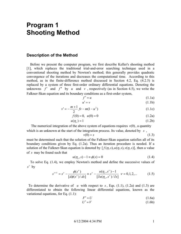
Program 1
Shooting Method
Description of the Method
Before we present the computer program, we first describe Keller's shooting method
[1], which replaces the traditional trial-and-error searching technique used in a
conventional shooting method by Newton's method; this generally provides quadratic
convergence of the iterations and decreases the computational time. According to this
method, as in the finite-difference method discussed in Section 4.2, Eq. (4.2.5) is
replaced by a system of three first-order ordinary differential equations. Denoting the
unknowns f ′ and f ′′ by u and v , respectively (as in Section 4.5), we write the
Falkner-Skan equation and its boundary conditions as a first-order system,
f′=u
(1.1a)
u′ = v
(1.1b)
m +1
v′ = −
fv − m(1 − u 2 )
(1.1c)
2
f (0) = 0, u (0) = 0
(1.2a)
u (η e ) = 1
(1.2b)
The numerical integration of the above system of equations requires v(0) , a quantity
which is an unknown at the start of the integration process. Its value, denoted by s ,
v(0) = s
(1.3)
must be determined such that the solution of the Falkner-Skan equation satisfies all of its
boundary conditions given by Eq. (1.2a). Thus an iteration procedure is needed. If a
solution of the Falkner-Skan equation is denoted by [ f (η , s ), u (η , s ), v(η , s )] , then a value
of s may be found such that
u (η e , s ) − 1 ≡ φ ( s ) = 0
(1.4)
To solve Eq. (1.4), we employ Newton's method and define the successive values of
ν
s by
u (η e , sν ) − 1
φ ( sν )
ν +1
ν
ν
s =s −
≡s −
ν = 0,1, 2,...
(1.5)
[dφ ( sν ) / ds ]
[∂u (η e , sν ) / ∂s ]
To determine the derivative of u with respect to s , Eqs. (1.1), (1.2a) and (1.3) are
differentiated to obtain the following linear differential equations, known as the
variational equations, for Eq. (1.1):
F′ = U
(1.6a)
′
U =V
(1.6b)
6/12/2004 4:34 PM
1
V′ = −
and the initial conditions,
m +1
( fV + vF ) + 2muU
2
F (0) = 0, U (0) = 0, V (0) = 1
(1.6c)
(1.7)
Here
∂f
∂u
∂v
(1.8)
, U (η , s) ≡ , V (η , s) ≡
∂s
∂s
∂s
Once a solution of the Falkner-Skan equation is obtained subject to Eqs. (1.2a) and
(1.3), and a solution of the variational equations (1.6), subject to Eqs. (1.7), u (η e , sν ) and
F (η , s ) ≡
U (η e , sν ) is known, then the next approximation to v(0) , namely sν +1 can be computed
from Eq. (1.5). The solution procedure is repeated until convergence when
| sν +1 − sν |< ε
(1.9)
where ε is a convergence parameter.
Computer Program
We now describe the computer program for solving the Falkner-Skan equation for a
specified value of m using the shooting method discussed above. While several
integration methods can be used to solve the initial value problem, here, because of its
simplicity, a fourth-order Runge-Kutta method is used.
The computer program consists of a main program containing the logic of the
computations which has three subroutines: STNDRD, VARS and RKM. The following is
a description of the computer program and its subroutines.
MAIN
Contains the input data, the boundary-layer grid, the logic of the
numerical scheme, the number of iterations performed, and the output,
which consists of the profiles f , u , v as a function of η and the
dimensionless displacement and momentum thickness parameters δ 1∗
and θ1 , respectively
ηe
δ 1∗ = ∫ (1 − f ′)dη = η e − f e
0
ηe
θ1 = ∫ f ′(1 − f ′)dη
0
The input data are similar to the input data described for the finite-difference
boundary-layer method BLP2 in Program 3, with NXT, ITMAX, ∆ X, S(1), ETAINF,
EPS corresponding to the total number of x -stations, maximum iteration number, ∆η increment, v(0) = S (1) , η e and convergence criterion, which is usually taken as 10 −5 or
10 −6 .
6/12/2004 4:34 PM
2
Program Main
C
PROGRAM MAIN
COMMON/SHARE/F(101),U(101),V(101),PNX1,NP,DX,NX,ETA(101),P(15),
1
S(15),PHI,ETAINF,DERWRS
C-------------------------------------------------------------------C INPUT
READ(5,8000) NXT,ITMAX,DX,S(1),ETAINF,EPS
READ(5,8100) (P(I),I=1,NXT)
C TOTAL NUMBER OF GRID POINTS, NP
NP = ETAINF/DX +1.1
NX = 1
C INITIAL VALUE OF INDEPENDENT VARIABLE
60 ETA(1) = 0.0
WRITE(6,9300) NX,P(NX),S(NX)
WRITE(6,9050)
IT = O
PNX1 = -0.5*(P(NX)+1.0)
C
90 IT = IT+1
IF (IT .LE. ITMAX) GO TO 95
WRITE(6,9000)
GO TO 400
C
95 CALL STNDRD
CALL VARS
TERM = PHI/DERWRS
WRITE(6,9060) S(NX),TERM
S(NX) = S(NX)-TERM
C
C CHECK FOR CONVERGENCE
IF (ABS(TERM) .GT. EPS) GO TO 90
CALL STNDRD
S(NX+1) = S(NX)
C OUTPUT
400 WRITE(6,9070)
DO 2 J=1,NP,8
2 WRITE(6,9100) J,ETA(J),F(J),U(J),V(J)
DELST1 = ETA(NP) - F(NP)
THETA1 = (S(NX)-P(NX)*DELST1)/(1.5*P(NX)+0.5)
WRITE(6,9200) DELST1,THETA1
C
NX = NX+1
IF (NX .LE. NXT .AND. IT .LE. ITMAX) GO TO 60
STOP
C---------------------------------------------------------------8000 FORMAT(2I3,4F10.0)
8100 FORMAT(F10.0)
9000 FORMAT(1H ,25HITERATIONS EXCEED MAXIMUM)
9050 FORMAT(1H ,11X,1HS,13X,3H-DS)
9060 FORMAT(1H ,5X,2E14.6)
9070 FORMAT(1H ,2X,1HJ,4X,3HETA,9X,1HF,13X,1HU,13X,1HV/)
9100 FORMAT(1H ,I3,F10.4,4E14.6)
9200 FORMAT(1H ,7HDELST1=,E14.6,3X,7HTHETA1=,E14.6//)
9300 FORMAT(1H ,3HNX=,I3,5X,2HP=,F10.6,5X,2HS=,F10.6)
END
6/12/2004 4:34 PM
3
Subroutine STNDRD
STDRD
Defines the boundary and initial conditions given by Eqs. (1.2a) and
(1.3) at the wall and the system of equations given by Eq. (1.1). Also,
s in Eq. (1.4a) is computed.
SUBROUTINE STNDRD
COMMON/SHARE/F(101),U(101),V(101),PNX1,NP,DX,NX,ETA(101),P(15),
1
S(15),PHI,ETAINF,DERWS
DIMENSION C(3),B(3),Z(3),G(12)
C-------------------------------------------------------------------C DEFINITION OF FIRST-ORDER SYSTEM
C INITIAL VALUES OF DEPENDENT VARIABLES
N = 3
X = 0.0
IS = 0
B(1) = 0.0
B(2) = 0.0
B(3) = S(NX)
F(1) = B(1)
U(1) = B(2)
V(1) = B(3)
C
DO 100 J=2,NP
DO 110 LL=1,4
C(1) = B(2)
C(2) = B(3)
C(3) = PNX1*B(1)*B(3)-P(NX)*(1.0-B(2)**2)
110 CALL RKM(X,B,C,DX,N,Z,G,IS)
C
C SAVE CURRENT VALUES
F(J) = B(1)
U(J) = B(2)
V(J) = B(3)
100 ETA(J) = X
PHI = U(NP)-1.0
RETURN
END
Subroutine VARS
VARS
Defines the variational equations and their initial conditions given by
Eqs. (1.6) and (1.7). U (η e , sν ) in Eq. (1.5) is computed here.
SUBROUTINE VARS
COMMON/SHARE/F(101),U(101),V(101),PNX1,NP,DX,NX,ETA(101),P(15),
1
S(15),PHI,ETAINF,DERWRS
DIMENSION C(3),B(3),Z(3),G(12)
C-------------------------------------------------------------------C INITIAL VALUES OF DEPENDENT VARIABLES
6/12/2004 4:34 PM
4
N = 3
X = 0.0
IS = 0
B(1) = 0.0
B(2) = 0.0
B(3) = 1.0
FF = F(1)
UU = U(1)
VV = V(1)
C SOLUTION FOR GIVEN F,FP,FPP PROFILES
DO 100 J=2,NP
FJ = F(J)
UJ = U(J)
VJ = V(J)
DO 10 LL=1,4
GO TO (4,2,4,3),LL
2 FF = (FF+FJ)/2.0
UU = (UU+UJ)/2.0
VV = (VV+VJ)/2.0
GO TO 4
3 FF = FJ
UU = UJ
VV = VJ
4 C(1) = B(2)
C(2) = B(3)
C(3) = PNX1*(VV*B(1)+FF*B(3))+2.0*P(NX)*B(2)*UU
10 CALL RKM(X,B,C,DX,N,Z,G,IS)
100 CONTINUE
C
DERWRS = B(2)
RETURN
END
Subroutine RKM
RKM contains the Runge-Kutta method, which is of fourth order in ∆η . It integrates
any system of first-order quasi-linear simultaneous ordinary differential equations and is
not specialized to the Falkner-Skan system. To describe this method, consider a firstorder differential equation of the form
dy
= f ( x, y )
(1.10)
dx
subject to the prescribed initial condition y = y0 when x = x0 . According to the
commonly used fourth-order Runge-Kutta method, the solution of Eq. (4A.10) is given
by
1
yn+1 = yn + (k1 + 2k2 + 2k3 + k4 )
(1.11)
6
where, with h = xn+1 − xn = ∆x ,
6/12/2004 4:34 PM
5
k1 = hf ( x n , y n )
k 2 = hf ( x n + 12 h, y n + 12 k1 )
k 3 = hf ( x n + 12 h, y n + 12 k 2 )
k 4 = hf ( x n + h, y n + k 3 )
(1.12)
Thus, in each step in  (or x ), RKM must be called four times. The arguments X to
IS have the following explanation.
• The independent variable  . The initial value for X must be input.
• A floating point array that is dimensioned N . The B(I ) are the current values of the
dependent variables. For example,
f
B (1)
u = B ( 2)
v
B (3)
Initial values f (0) , u0 , and v(0) must be input.
DX
A floating point array that is dimensioned N . The ( CI ) are the current
values of derivatives. These values are supplied to RKM through the
argument list. For example,
F C (1)
U = C (2)
V C (3)
DX
N
F
The increment in  . DX must be input
The number of simultaneous equations to be integrated.
A floating point array used by the subroutine to store values of the array
B . F is dimensioned N .
A floating array that contains intermediate values computed by the
subroutine. Four entries of G are used to compute one entry of B . G
is dimensioned 4 ∗ N .
A code variable that must be set to zero to initialize the subroutine. IS is
automatically stepped through the values 1, 2, 3 and 4 and is reset to zero
by the subroutine after user variables for X and the array B are
computed. The four entries to RKM are, in effect, four improved
estimates of the required integral over the interval DX .
G
IS
SUBROUTINE RKM(A,B,C,DX,N,F,G,IS)
DIMENSION C(N),B(N),F(N),G(4*N)
C-------------------------------------------------------------------IS = IS+1
GO TO (10,30,60,80), IS
C FIRST ENTRY
10 E = A
DO 20 I=1,N
6/12/2004 4:34 PM
6
F(I) = B(I)
G(4*I-3) = C(I)*DX
20 B(I) = F(I)+G(4*I-3)/2.0
GO TO 50
C SECOND ENTRY
30 DO 40 I=1,N
G(4*I-2) = C(I)*DX
40 B(I) = F(I)+G(4*I-2)/2.0
50 A = E+DX/2.0
GO TO 100
C THIRD ENTRY
60 DO 70 I=1,N
G(4*I-1) = C(I)*DX
70 B(I) = F(I)+G(4*I-1)
A = E+DX
GO TO 100
C FOURTH ENTRY
80 DO 90 I=1,N
G(4*I) = C(I)*DX
B(I) = G(4*I-3)+2.0*(G(4*I-2)+G(4*I-1))
90 B(I) = (B(I)+G(4*I))/6.0+F(I)
IS = 0
100 RETURN
END
Applications
To demonstrate the applications of the computer program and its output, we present
results for Blasius similar flow m = 0 , which corresponds to NXT = 1 . We take
ITMAX = 6 , ∆η -increment (DX) 0.1, wall shear (1) at NX = 1 as 0.300, η e as 8 and
convergence parameter as 10 −6 .
The output presented below shows that the profiles f j , u j , v j as functions of η j
and j together with the rate of convergence of the solutions and dimensionless
boundary-layer parameters δ 1∗ and θ1 for each value of m .
The results for m = 0 show that, for an assumed wall shear value of 0.3, the rate of
convergence of the solutions in quadratic, requiring only three iterations. To obtain
solutions for m = 0.5 , we have used increments of ∆m = 0.1 . Again, the convergence
rate is quadratic. Similar results are also obtained for m = 1 . Results are only presented
for m = 0 , 0.5 and 1.0.
NX=
1
J
P= 0.000000
S= 0.300000
S
-DS
0.300000E+00 -0.315214E-01
0.331521E+00 -0.537911E-03
0.332059E+00 -0.296956E-07
ETA
F
U
1
0.0000
0.000000E+00
0.000000E+00
6/12/2004 4:34 PM
V
0.332059E+00
7
9
0.8000 0.106109E+00 0.264711E+00 0.327391E+00
17
1.6000 0.420323E+00 0.516760E+00 0.296665E+00
25
2.4000 0.922295E+00 0.728986E+00 0.228093E+00
33
3.2000 0.156910E+01 0.876086E+00 0.139128E+00
41
4.0000 0.230576E+01 0.955522E+00 0.642340E-01
49
4.8000 0.308534E+01 0.987794E+00 0.218711E-01
57
5.6000 0.388031E+01 0.997482E+00 0.543197E-02
65
6.4000 0.467938E+01 0.999616E+00 0.980645E-03
73
7.2000 0.547925E+01 0.999960E+00 0.128584E-03
81
8.0000 0.627924E+01 0.100000E+01 0.122445E-04
DELST1= 0.172075E+01
THETA1= 0.664119E+00
NX=
1
J
P= 0.500000
S= 0.817270
S
-DS
0.817270E+00 -0.899329E-01
0.907203E+00 0.746350E-02
0.899739E+00 0.226980E-04
0.899717E+00 -0.125888E-06
ETA
F
U
V
1
0.0000 0.000000E+00 0.000000E+00 0.899717E+00
9
0.8000 0.245793E+00 0.563205E+00 0.516792E+00
17
1.6000 0.827465E+00 0.852277E+00 0.227309E+00
25
2.4000 0.156199E+01 0.963375E+00 0.716724E-01
33
3.2000 0.234773E+01 0.993629E+00 0.154319E-01
41
4.0000 0.314556E+01 0.999247E+00 0.220024E-02
49
4.8000 0.394534E+01 0.999941E+00 0.203881E-03
57
5.6000 0.474532E+01 0.999997E+00 0.122146E-04
65
6.4000 0.554532E+01 0.100000E+01 0.554850E-06
73
7.2000 0.634532E+01 0.100000E+01 0.910765E-07
81
8.0000 0.714532E+01 0.100000E+01 0.688662E-07
DELST1= 0.854673E+00
THETA1= 0.377904E+00
NX=
J
1
P= 1.000000
S= 1.173530
S
-DS
0.117353E+01 -0.175270E+00
0.134880E+01 0.756893E-01
0.127311E+01 0.327164E-01
0.124039E+01 0.742014E-02
0.123297E+01 0.387354E-03
0.123259E+01 0.581049E-06
ETA
F
U
V
1
0.0000 0.000000E+00 0.000000E+00 0.123259E+01
9
0.8000 0.312424E+00 0.685937E+00 0.525132E+00
17
1.6000 0.979781E+00 0.932347E+00 0.147353E+00
25
2.4000 0.175525E+01 0.990548E+00 0.260216E-01
33
3.2000 0.255233E+01 0.999185E+00 0.275514E-02
41
4.0000 0.335211E+01 0.999957E+00 0.168261E-03
49
4.8000 0.415210E+01 0.999997E+00 0.519110E-05
57
5.6000 0.495210E+01 0.999998E+00 -0.660768E-06
65
6.4000 0.575210E+01 0.999997E+00 -0.864673E-06
73
7.2000 0.655210E+01 0.999997E+00 -0.934394E-06
81
8.0000 0.735209E+01 0.999996E+00 -0.109396E-05
DELST1= 0.647902E+00
THETA1= 0.292342E+00
6/12/2004 4:34 PM
8
Source Code, input data and test cases
6/12/2004 4:34 PM
9