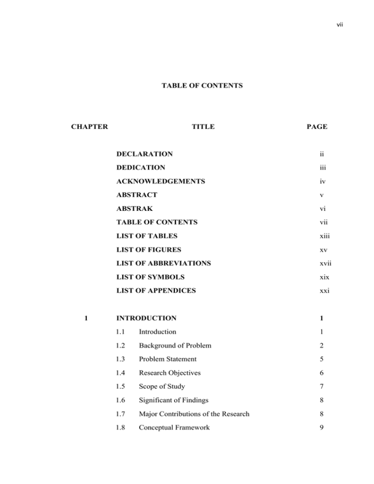
TABLE OF CONTENTS CHAPTER TITLE PAGE
advertisement

vii
TABLE OF CONTENTS
CHAPTER
1
TITLE
PAGE
DECLARATION
ii
DEDICATION
iii
ACKNOWLEDGEMENTS
iv
ABSTRACT
v
ABSTRAK
vi
TABLE OF CONTENTS
vii
LIST OF TABLES
xiii
LIST OF FIGURES
xv
LIST OF ABBREVIATIONS
xvii
LIST OF SYMBOLS
xix
LIST OF APPENDICES
xxi
INTRODUCTION
1
1.1
Introduction
1
1.2
Background of Problem
2
1.3
Problem Statement
5
1.4
Research Objectives
6
1.5
Scope of Study
7
1.6
Significant of Findings
8
1.7
Major Contributions of the Research
8
1.8
Conceptual Framework
9
viii
1.8.1
Stochastic Job Shop Scheduling Problems:
Assumptions
1.8.2
Problem Representation and Stochastic
Precedence Networks
10
1.8.3
Modeling Uncertainty in Scheduling
11
1.8.4
Stochastic Performance measure and Objective
Functions
1.8.5
1.9
2
10
12
Stochastic Scheduling Complexity and
Optimization
13
1.8.6
Metaheuristics
14
1.8.7
Simulation
15
Outline of the Thesis
16
LITERATURE REVIEW
18
2.1
Introduction
18
2.2
Deterministic Job Shop Scheduling Problem
18
2.2.1
Schedules, Sequences and Timetables
21
2.2.2
Types of Schedules
22
2.2.3
The Disjunctive Graph Representation
24
2.2.3.1 Representing Scheduling Problems
24
2.2.3.2 Representing Solutions
25
Schedules Generation Techniques
28
2.3
Stochastic Job Shop Scheduling Problem
30
2.4
PERT Network and Solution Representation
32
2.5
Combining Solution Techniques with Simulation
33
2.6
Solution Methods for Stochastic Scheduling
34
2.6.1
Mathematical Programming Approaches
35
2.6.1.1 Lagrangian Relaxation
35
2.6.1.2 Dynamic Programming
35
2.2.4
ix
2.6.2
3
2.6.1.3 Branch and Bound
36
Heuristics
37
2.6.2.1 Priority Dispatching Rules
38
2.6.2.2 Shifting Bottleneck Procedure
40
2.6.2.3 Simulated Annealing
40
2.6.2.4 Tabu Search
45
2.6.2.5 Genetic Algorithms
47
2.6.2.6 Ant Colony Optimization
48
2.7
Previous Works on SJSSPs
49
2.8
Benchmark Problems
52
2.9
Summary
54
METHODOLOGY
56
3.1
Introduction
56
3.2
Simulated Annealing Background
56
3.2.1
Algorithm’s Parameters and Components
57
3.2.1.1 Annealing Schedules
58
3.2.1.2 Initial Temperature
59
3.2.1.3 Final Temperature
59
3.2.1.4 Length of Markov Chain
59
3.2.1.5 Random Number Generator
60
Extension of the algorithm for Stochastic Problems
61
3.3.1
Problem Representation
63
3.3.2
Generating an Initial Solution
64
3.3.3
The Neighborhood Structures
65
3.3
3.3.4 Comparison between Current Solution and
Candidate Solution
68
3.3.5
Determination of Best Cost Function Value
69
3.3.6
Sampling Schedule
69
x
3.3.7
3.4
4
Cooling Schedule for SSA
Summary
70
70
SIMULATION-BASED SIMULATED ANNEALING FOR
JOB SHOP SCHEDULING PROBLEM WITH RANDOM
PROCESSING TIMES
71
4.1
Introduction
71
4.2
Simulation-based Simulated Annealing for SJSSP
72
4.2.1
Objective Function Computation
72
4.2.2
Determination of Sample Size
72
4.2.3
Simple Monte Carlo Sampling
74
4.2.4
Common Random Numbers
74
4.2.5
Descriptive Sampling
75
4.2.6
Evaluation of Statistics
78
4.2.6.1 Estimation of the Expected Makespan
78
4.2.6.2 Estimation of the α-quantile of Makespan
79
4.3
5
Cooling Schedules
81
4. 3.1 Conventional Cooling Schedule
81
4.3.2
Adaptive Temperature Schedule
81
4.3.3
Constant Temperature
84
4.4
Simulated Annealing with Confidence Interval
85
4.5
Summary
88
EXPERIMENTS AND ANALYSIS ON EXPECTED
MAKESPAN
90
5.1
Introduction
90
5.2
Computational Set Up
90
5.2.1
Problem Generation
92
5.2.2
Initial Solution
93
xi
5.3
5.4
5.2.3
Neighborhood Structure
93
5.2.4
Parameters Tuning
94
5.2.4.1 The Cooling Schedules
94
5.2.4.2 Number of Simulation Replications
95
Simulation Results on Expected Makespan
101
5.3.1
Straightforward Implementation of PDSA
101
5.3.2
Makespan Distribution of Various Solution
106
SSA as Planning Tool
110
5.4.1
Impact of Additional Ingredients
116
5.4.1.1 SSA with Adaptive Temperature Control
116
5.4.1.2 SSA with Constant Temperature
119
5.4.1.3 SSA with Confidence Interval
122
Average Performance Comparison
124
5.4.2
6
5.5
Comparison of SSA Variants with other Algorithms
126
5.6
Summary
127
MAKESPAN QUANTILES AND MAKESPAN
DISTRIBUTIONS FOR STOCHASTIC JOB SHOP
SCHEDULING PROBLEM
129
6.1
Introduction
129
6.2
Experiments on α-quantile of Makespan
130
6.2.1
130
Results and Analysis
6.3
Correlations Analysis
134
6.4
Makespan Distribution
137
6.4.1
Fitting Distribution
138
6.4.2
Normality Test
139
6.4.2.1 Choosing between One or More Fitted
Distributions
6.5
Summary
140
143
xii
7
SUMMARY AND FUTURE RESEARCH
144
7.1
Summary
144
7.2
Future Research
147
REFERENCES
149
Appendices A-C
156-159
xiii
LIST OF TABLES
TABLE NO.
TITLE
PAGE
2.1
An example of 3x3 job shop scheduling problem
20
2.2
6x6 problem instance with exponential processing times
32
2.3
The description of some priority dispatching rules
39
2.4
Muth and Thompson’s 6-by-6 problem (FT06)
53
2.5
Muth and Thompson’s 10-by-10 problem (FT10)
53
2.6
Muth and Thompson’s 10-by-10 problem (FT20)
54
3.1
6x6 problem instance with exponential distributed
processing times
63
3.2
A solution to a 6x6 SJSSP
64
4.1
Stored values for a uniform distribution U (1,5) and n = 10
76
4.2
Stored values for an exponential distribution Exp(3) and n = 10
77
5.1
A summary of algorithms for the SJSSP
91
5.2
Summary of experimental factors
93
5.3
Summary of results comparing simple random sampling (SRS)
with descriptive sampling (DS) for different simulation
with CV =0.144
5.4
97
Summary of results comparing simple random sampling (SRS)
with descriptive sampling (DS) for different simulation
with CV =1
98
5.5
Summary of Parameters Setting
100
5.6
Computational results of PDSA algorithm initialized from
RANDOM dispatching rule
103
xiv
5.7
Performances of the 11 Benchmark Job Shop Scheduling
Problems
5.8
Summary statistics on tight and loose sequences for FT06
and FT10 with CV1
5.9
107
Summary statistics on tight and loose sequences for FT06
and FT10 with CV3
5.11
107
Summary statistics on tight and loose sequences for FT06
and FT10 with CV2
5.10
106
108
Summary statistics on tight and loose sequences for FT06
and FT10 with CV4
108
5.12
Computational results of SSA algorithm on FT06
110
5.13
Computational results of SSA algorithm
114
5.14
Computational results of SSA _ADPT
118
5.15
Ten high, low and medium temperature random trials
for FT06
120
5.16
Computational results of SSA _CONT
121
5.17
Computational results of variants of SSA with
Confidence Interval
122
5.18
Mean performance of SSA variants on 10-by-10 instances
127
6.1
Average qα(Cmax) generated by the SSA in 30 runs
134
6.2
Average coefficients of determination for the relationship
between E(Cmax) and qα(Cmax) on FT10, ABZ5, ABZ6 and
LA16 instances
136
6.3
Goodness of fit summary FT10
141
6.4
Fitting Results for FT10
142
6.5
Goodness-of-fit for normality on all test instances
142
xv
LIST OF FIGURES
FIGURE NO.
TITLE
PAGE
1.1
Conceptual Frameworks
9
1.2
Histogram for Makespan of ABZ06
15
2.1
Gantt chart of the feasible solution of the 3x3 problem
22
2.2
Active schedule
23
2.3
Disjunctive Graph for 3x3 instance (Table 2.1)
25
2.4
The example of JSP instance (Table 2.1) with three
feasible solutions
26
3.1
An illustration of N1 neighborhood
67
5.1
Estimated expected makespan for different processing
time variability as a function of sample size for FT10
5.2
99
Standard deviation of makespan distribution for different
processing time variability as a function of sample size
for FT10
5.3
Relationship between expected makespan and processing
times variability
5.4
104
Relationship between coefficient of variation of the makespan
and processing time variability
5.6
104
Relationship between makespan variance and processing
time variability
5.5
100
Best sequences generated by SSA algorithm for the
FT06 instance with different processing time variability
105
xvi
(a) U1 (b) U2 (c) U3 and (d) EX
5.7
111
Relationship between expected makespan and
pseudo deterministic makespan for FT06 with different
processing time variability (a) U1 (b) U2 (c) U3
and (d) EXP
112
5.8
Mean performance of SSA and PDSA
116
5.9
Mean performance of SSA variants on G1 instances
125
5.10
Mean performance of SSA variants on G2 instances
125
5.11
Mean performance of SSA variants on G3 instances
126
6.1
The best sequence q0.99 (Cmax ) generated by SSA for
ABZ6 with data coming from four variability levels
(a) CV1, (b) CV2, (c) CV3 and (d) CV
6.2
132
The scatter plots (the mean makespan is plotted on the
x-axis and the alpha quantile on the y-axis) of FT10
with four variability levels (a) CV1, (b) CV2, (c) CV3
and (d) CV4
6.3
6.4
135
Histogram of the different makespan realizations of a
solution for FT10 with (a) CV1 and (d) CV4
138
Probability Plot for LA16 with four variability levels
140
xvii
LIST OF ABBREVIATIONS
ACO
-
Ant Colony Optimization
BB
-
Branch and Bound
CDF
-
Cumulative Distribution Function
CI
-
Confidence Interval
CRN
-
Common Random Numbers
CV
-
coefficient of variation
DJSSP
-
Deterministic Job Shop Scheduling Problem
DP
-
Dispatching Rules
DS
-
Descriptive Sampling
GA
-
Genetic Algorithm
GT
-
Giffler and Thompson
JSSP
-
Job Shop Scheduling Problem
LL
-
Lower Limit (1 )100% confident limit
LPT
-
Longest Processing Time
LR
-
Lagrangian Relaxation
N1
-
Neighborhood structure of VanLaarhoven
N2
-
Neighborhood structure of Dell’Amico and Trubian
N3
-
Neighborhood structure of Novicki and Smutnicki
PD
-
Priority Dispatching
PDF
-
Probability density function
PDSA
-
Pseudo-deterministic simulated annealing
PERT
-
Project Evaluation and Review Technique
RANDOM
-
Random rule
xviii
SA
-
Simulated Annealing
SJSSP
-
Stochastic Job Shop Scheduling Problem
SPT
-
Shortest Processing Time
SSA
-
Simulation-based simulated annealing
SSA_ADPT
-
Simulation-based simulated annealing with adaptive
Temperature
SSA_ADPT_CI -
Simulation-based simulated annealing with adaptive
Temperature and confidence interval
SSA_CONT_CI -
Simulation-based simulated annealing with constant
And Confidence Interval
SSA_CI
-
Simulation-based simulated annealing with constant
with confidence interval
TS
-
Tabu Search
UL
-
Upper Limit (1 )100% confident limit
xix
LIST OF SYMBOLS
s
-
A solution of JSSP
Jj
-
Job j
Mi
-
Machine i
Oij
-
An operation of J j on M i
Cj
-
Completion time of J j
Sij
-
The length of the longest path from the start to the
completion of Oij
Tij
-
The length of the longest path from the completion
of Oij to the sink
{Oij }
-
A sequence of operation of J j on M i
Tk
-
Temperature at kth iteration
Tf
-
Final temperature
T0
-
Initial temperature
-
Date line
rj
-
Release time of J j
Fj
-
Flow time of J j
Lj
-
Lateness of J j
dj
-
Due date of J j
Tj
-
Tardiness of J j
Ej
-
Earliness of J j
xx
F
-
Total flow time
L
-
Total lateness
E
-
Total earliness
T
-
Total tardiness
Lmax
-
Maximum lateness
Tmax
-
Maximum tardiness
SM (Oij )
-
Machine successor of Oij
SJ (Oij )
-
Job successor of Oij
PM (Oij )
-
Machine predecessor Oij
PJ (Oij )
-
Job predecessor Oij
N (s)
-
Neighborhood structure of a solution s
N1
-
Neighborhood structure of VanLaarhoven
N2
-
Neighborhood structure of Dell’Amico and Trubian
N3
-
Neighborhood structure of Novicki and Smutnicki
Cmax
-
Makespan
Fˆ (C max ( s ))
-
An estimation of statistic of makespan for s
q (C max )
-
α-quantile of makespan
xxi
LIST OF APPENDICES
APPENDIX
TITLE
PAGE
A.1
Practical Processing Times Distributions
156
A.1.1
The Uniform Distribution
156
A.1.2
The Exponential Distribution
156
B
The Jensen Gap
158
C
Conference Papers
159


