Measure of Variability (Dispersion, Spread) Range
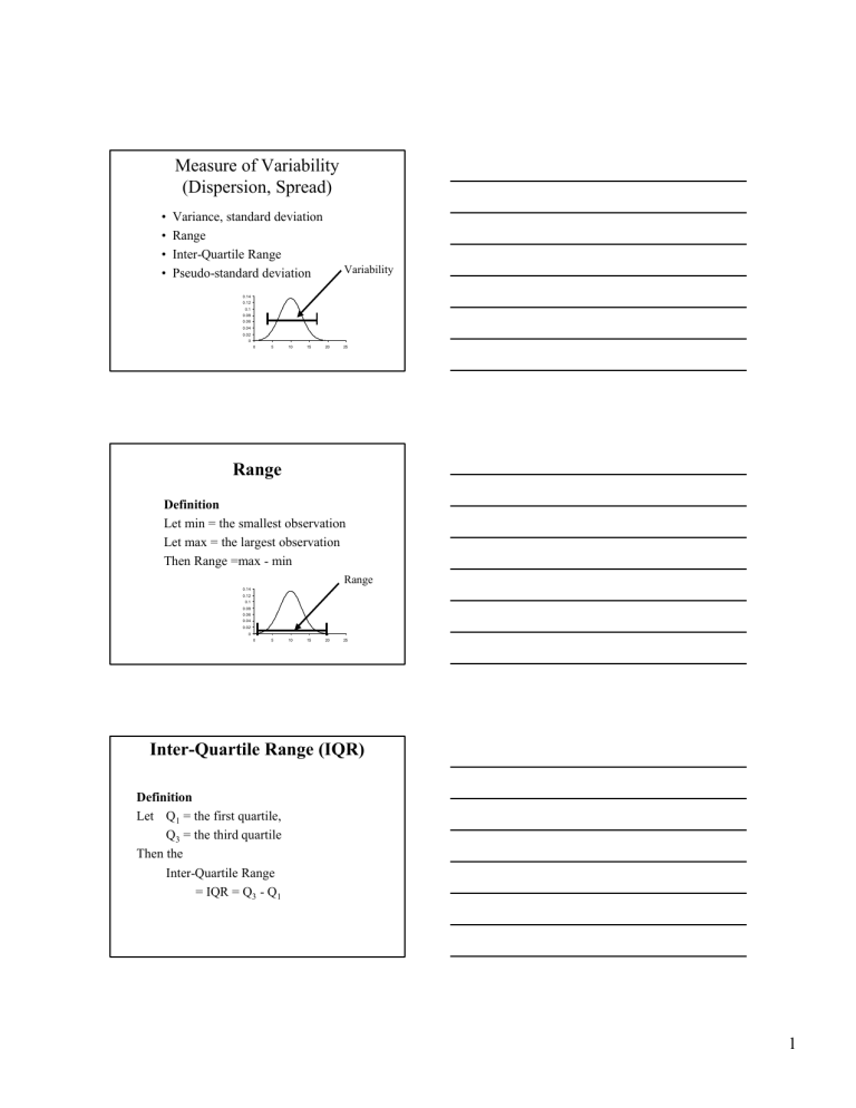
Measure of Variability
(Dispersion, Spread)
• Variance, standard deviation
• Range
• Inter-Quartile Range
• Pseudo-standard deviation
0.14
0.12
0.1
0.08
0.06
0.04
0.02
0
0 5 10 15 20 25
Variability
Range
Definition
Let min = the smallest observation
Let max = the largest observation
Then Range =max - min
Range
0.14
0.12
0.1
0.08
0.06
0.04
0.02
0
0 5 10 15 20 25
Inter-Quartile Range (IQR)
Definition
Let Q
1
= the first quartile,
Q
3
= the third quartile
Then the
Inter-Quartile Range
= IQR = Q
3
- Q
1
1
0.14
0.12
0.1
0.08
0.06
0.04
0.02
0
0
Inter-Quartile Range
50%
25%
5
Q
1
10
25%
Q
3
15 20 25
Example
The data Verbal IQ on n = 23 students arranged in increasing order is:
80 82 84 86 86 89 90 94
94 95 95 96 99 99 102 102
104 105 105 109 111 118 119
Example
The data Verbal IQ on n = 23 students arranged in increasing order is:
80 82 84 86 86 89 90 94 94 95 95 96 99 99 102 102 104 105 105 109 111 118 119 min = 80 Q
1
= 89 Q
2
= 96
Q
3
= 105 max = 119
2
Range
Range = max – min = 119 – 80 = 39
Inter-Quartile Range
= IQR = Q
3
- Q
1
= 105 – 89 = 16
Some Comments
• Range and Inter-quartile range are relatively easy to compute.
• Range slightly easier to compute than the
Inter-quartile range.
• Range is very sensitive to outliers (extreme observations)
Sample Variance
Let x
1
, x
2
, x
3
, … x n denote a set of n numbers.
Recall the mean of the n numbers is defined as: x
= i n
∑
=
1 x i n
= x
1
+ x
2
+ x
3
+ K + x n
−
1
+ x n n
3
The numbers d d
2 d d
1
3 n
=
=
= x
1 x
2
=
M x
3 x n
−
−
−
− x x x x are called deviations from the the mean
The sum n ∑ i
=
1 d i
2 = i n ∑
=
1
( x i
− x
)
2 is called the sum of squares of deviations from the the mean.
Writing it out in full: d
1
2 + d
2
2 + d
3
2 or
+ L + d n
2
( x
1
− x
) ( x
2
− x
)
2 + L + ( x n
− x
)
2
The Sample Variance
Is defined as the quantity: n ∑ i
=
1 n
− d
1 i
2
= i n ∑
=
1
( x i
− x
)
2 n
−
1 and is denoted by the symbol s 2
4
Example
Let x
1
, x
2
, x
3
, x
3
, x
4
, x
5 denote a set of 5 denote the set of numbers in the following table.
i 1 2 3 4 5 x i
10 15 21 7 13
Then
5
∑
i
=
1 x i
= x
1
+ x
2
+ x
3
+ x
4
+ x
5
= 10 + 15 + 21 + 7 + 13 and x
= i n
∑
=
1 x i n
= 66
= x
1
+ x
2
+ x
3
+ K + x n
−
1
+ x n n
=
66
5
=
13 .
2
The deviations from the mean d
1
, d
2
, d
3
, d
4
, d
5 are given in the following table.
i 1 2 3 4 5 x i
10 15 21 7 13 d i
-3.2
1.8
7.8
-6.2 -0.2
5
The sum i n ∑
=
1
=
( d
− i
2
3
=
.
2 i n ∑
=
1
( x i
1 .
8
− x
)
2
) ( ) ( ) (
−
6 .
2
) (
−
0 .
2
)
2
=
10 .
24
+
3 .
24
+
=
112 .
80
60 .
84
+
38 .
44
+
0 .
04 and s 2
= i n ∑
=
1
( x i
− x
)
2 n
−
1
=
112 .
8
4
=
28 .
2
The Sample Standard Deviation s
Definition: The Sample Standard Deviation is defined by: s
= i n ∑
=
1 n
− d i
2
1
= n ∑ i
=
1
( x i
− x
)
2 n
−
1
Hence the Sample Standard Deviation, s, is the square root of the sample variance.
In the last example s
= s
2 = i n ∑
=
1
( x i
− x
)
2 n
−
1
=
112 .
8
=
4
28 .
2
=
5 .
31
6
Interpretations of s
• In Normal distributions
– Approximately 2/3 of the observations will lie within one standard deviation of the mean
– Approximately 95% of the observations lie within two standard deviations of the mean
– In a histogram of the Normal distribution, the standard deviation is approximately the distance from the mode to the inflection point
0.14
0.12
0.1
0.08
0.06
0.04
0.02
0
0
Mode
Inflection point
5 s
10 15 20 25
2/3 s s
7
2s
Example
A researcher collected data on 1500 males aged 60-65.
The variable measured was cholesterol and blood pressure.
– The mean blood pressure was 155 with a standard deviation of 12.
– The mean cholesterol level was 230 with a standard deviation of 15
– In both cases the data was normally distributed
Interpretation of these numbers
• Blood pressure levels vary about the value
155 in males aged 60-65.
• Cholesterol levels vary about the value 230 in males aged 60-65.
8
• 2/3 of males aged 60-65 have blood pressure within 12 of 155. Ii.e. between 155-12 =143 and 155+12 = 167.
• 2/3 of males aged 60-65 have Cholesterol within 15 of 230. i.e. between 230-15 =215 and 230+15 = 245.
• 95% of males aged 60-65 have blood pressure within 2(12) = 24 of 155. Ii.e. between 155-24 =131 and 155+24 = 179.
• 95% of males aged 60-65 have Cholesterol within 2(15) = 30 of 230. i.e. between 230-
30 =200 and 230+30 = 260.
A Computing formula for:
Sum of squares of deviations from the the mean : i n ∑
=
1
( x i
− x
)
2
The difficulty with this formula is that x will have many decimals.
The result will be that each term in the above sum will also have many decimals.
9
The sum of squares of deviations from the the mean can also be computed using the following identity: n ∑ i
=
1
( x i
− x
)
2 = n ∑ i
=
1 x i
2 − n ∑ i
=
1 x i
2 n
To use this identity we need to compute: n ∑ i
=
1 x i
= x
1
+ x
2
+ L + x n and i n ∑
=
1 x i
2 = x
1
2 + x
2
2 + L + x n
2
Then: n ∑ i
=
1
( x i
− x
)
2 = n ∑ i
=
1 x i
2 −
n ∑ i
=
1 n x i
2 and s
2 = i n ∑
=
1
( x i
− x
)
2 n
−
1
= n ∑ i
=
1 x i
2 − n
−
1 n ∑ i
=
1 x i n
2
10
and s
= i n ∑
=
1
( x i
− x
)
2 n
−
1
= i n ∑
=
1 x i
2 − n
−
1 i n ∑
=
1 x i
2 n
Example
The data Verbal IQ on n = 23 students arranged in increasing order is:
80 82 84 86 86 89 90 94
94 95 95 96 99 99 102 102
104 105 105 109 111 118 119 i n ∑
=
1 x i
= 80 + 82 + 84 + 86 + 86 + 89
+ 90 + 94 + 94 + 95 + 95 + 96
+ 99 + 99 + 102 + 102 + 104 n ∑ i
=
1 x i
2
+ 105 + 105 + 109 + 111 + 118
+ 119 = 2244
= 80 2 + 82 2 + 84 2 + 86 2 + 86 2 + 89 2
+ 99 2
+ 90 2
+ 99 2
+ 94 2
+ 102 2
+ 94 2
+ 102
+ 95
2
2 + 95
+ 104 2
2 + 96 2
+ 105 2 + 105 2 + 109 2 + 111 2
+ 118 2 + 119 2 = 221494
11
Then: n ∑ i
=
1
( x i
− x
)
2 = n ∑ i
=
1 x i
2 − n ∑ i
=
1 x i
2 n
=
221494
−
(
2244
)
2
23
=
2557 .
652 and s
2
=
= i n ∑
=
1
( x i
− x
)
2
221494
−
( n
−
1
2244
)
2
23
22
= i n ∑
=
1 x i
2 −
i n ∑
=
1 n x i n
−
1
2
=
2557 .
652
=
116 .
26
22
Also s
= i n ∑
=
1
( x i
− x
)
2 n
−
1
= n ∑ i
=
1 x i
2 −
n ∑ i
=
1 x i n
2 n
−
1
=
221494
−
(
2244
)
2
23
22
=
2557 .
652
=
22
116 .
26
=
10 .
782
12
A quick (rough) calculation of s
s
≈
Range
4
The reason for this is that approximately all
(95%) of the observations are between and x
+
2 s .
x
−
2 s
Thus max
≈ x
+
2 s and Range
= max
− and min min
≈
( x
≈
+ x
−
2 s
2 s .
) ( x
−
2 s
)
.
=
Hence s
≈
Range
4 s
4
Example
Verbal IQ on n = 23 students min = 80 and max = 119 s
≈
119 80
=
39
=
9 .
75
4 4
This compares with the exact value of s which is 10.782.
The rough method is useful for checking your calculation of s.
The Pseudo Standard Deviation (PSD)
Definition: The Pseudo Standard Deviation
(PSD) is defined by:
PSD
=
IQR
1 .
35
=
InterQuart ile Range
1 .
35
13
Properties
• For Normal distributions the magnitude of the pseudo standard deviation ( PSD ) and the standard deviation ( s ) will be approximately the same value
• For leptokurtic distributions the standard deviation
( s ) will be larger than the pseudo standard deviation ( PSD )
• For platykurtic distributions the standard deviation
( s ) will be smaller than the pseudo standard deviation ( PSD )
Example
Verbal IQ on n = 23 students
Inter-Quartile Range
= IQR = Q
3
- Q
1
= 105 – 89 = 16
Pseudo standard deviation
=
PSD
=
IQR
1 .
35
=
16
1 .
35
=
11 .
85
This compares with the standard deviation s
=
10 .
782
• An outlier is a “wild” observation in the data
• Outliers occur because
– of errors (typographical and computational)
– Extreme cases in the population
• We will now consider the drawing of boxplots where outliers are identified
14
To Draw a Box Plot we need to:
• Compute the Hinge (Median, Q
2
) and the
Mid-hinges (first & third quartiles – Q
1 and Q
3
)
• To identify outliers we will compute the inner and outer fences
• Lower inner fence
• f
1
= Q
1
- (1.5)IQR
Lower outer fence
F
1
= Q
1
- (3)IQR
Upper outer fence
F
2
= Q
3
+ (3)IQR
Lower inner fence f
1
= Q
1
- (1.5)IQR
Upper inner fence f
2
= Q
3
+ (1.5)IQR
15
• Observations that are between the lower and upper fences are considered to be nonoutliers.
• Observations that are outside the inner fences but not outside the outer fences are considered to be mild outliers.
• Observations that are outside outer fences are considered to be extreme outliers.
• mild outliers are plotted individually in a box-plot using the symbol
• extreme outliers are plotted individually in a box-plot using the symbol
• non-outliers are represented with the box and whiskers with
– Max = largest observation within the fences
– Min = smallest observation within the fences
Box-Whisker plot representing the data that are not outliers
Extreme outlier
Mild outliers
Inner fences
Outer fence
16
Measures of Shape
• Skewness
0.16
0.14
0.12
0.1
0.08
0.06
0.04
0.02
0
0 5 10 15 20 25
0.14
0.12
0.1
0.08
0.06
0.04
0.02
0
0 5 10 15 20 25
0.16
0.14
0.12
0.1
0.08
0.06
0.04
0.02
0
0 5 10 15 20 25
• Kurtosis
-3 -2 -1
0
0 1 2 3
0.14
0.12
0.1
0.08
0.06
0.04
0.02
0
0 5 10 15 20 25 -3 -2 -1
0
0 1 2 3
• Skewness – based on the sum of cubes i n ∑
=
1
( x i
− x
)
3
• Kurtosis – based on the sum of 4 th powers i n ∑
=
1
( x i
− x
)
4
17
