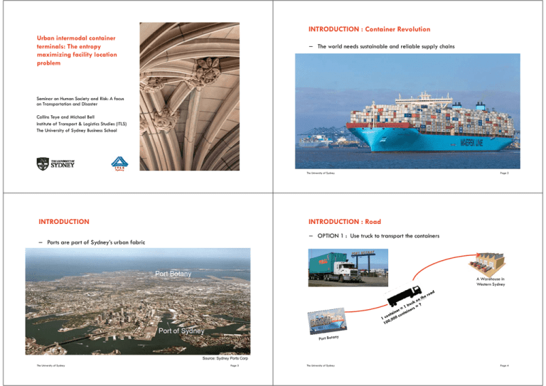
INTRODUCTION : Container Revolution
Urban intermodal container
terminals: The entropy
maximizing facility location
problem
– The world needs sustainable and reliable supply chains
Seminar on Human Society and Risk: A focus
on Transportation and Disaster
Collins Teye and Michael Bell
Institute of Transport & Logistics Studies (ITLS)
The University of Sydney Business School
The University of Sydney
Page 1
INTRODUCTION
The University of Sydney
Page 2
INTRODUCTION : Road
– OPTION 1 : Use truck to transport the containers
– Ports are part of Sydney’s urban fabric
A Warehouse in
Western Sydney
Source: Sydney Ports Corp
The University of Sydney
Page 3
The University of Sydney
Page 4
INTRODUCTION : Rail
INTRODUCTION : Intermodal Transport
─ OPTION II : Use trains to transport the containers
─ OPTION III : Use intermodal transport
Destination
Economies of scale
IMT
The University of Sydney
Page 5
INTRODUCTION : Key Research Question
The University of Sydney
Page 6
INTRODUCTION : Why is Location Important?
─ Where are the best places to locate IMTs?
Destination
─ The location of an IMT determines its viability
Determines the volume of cargo likely to use the IMT
Cargo volume is crucial to make an IMT viable
─ Influence rail mode share
The higher the use of the IMT the higher the share of rail
─ Determines the number of trucks that be taken off the road
Safer for other road users
Less road congestion, especially around the port
Less greenhouse gas emission, better environment, more sustainable
IMT
Where is the best place to
locate this terminal ?
Port
The University of Sydney
Page 7
The University of Sydney
Page 8
INTRODUCTION : Why the need for Intermodal Terminals?
INTRODUCTION : Advantages of IMTs
─ In Australia, containerised trade by volume is set to increase from 6.5 million
in 2011 to 11 million TEUs (containers) by 2020 (Shipping Australia, 2011)
─ Trucks currently accounts for over 86% of container trips to and from the
ports (Shipping Australia, 2011)
─ ADVANTAGE I: Economies of scale of rail
─ Rail has high carrying capacity, and
─ The larger the volume the cheaper to it is to use rail
─ Poor Management of empty containers: import, export imbalance
─ Congestion around ports with safety & environmental related problems
Destination
The University of Sydney
Page 9
INTRODUCTION : Advantages of IMTs
The University of Sydney
Page 10
INTRODUCTION : Advantages of IMTs
─ ADVANTAGE II: Economies of distance of rail
─ ADVANTAGE III: Accessibility
─ Less access by rail (can only reach few areas)
─ Flexible and easier access by trucks
─ Rail is cheaper for long distance trips
─ Rail is much greener and safer to other road users
Intermodal transport = Combined strengths of rail and truck
Unit cost
Truck
Break-even
distance
Rail = Exploit economies of scale + Economies of distance
Rail
Truck = Efficient and flexibility of local pick-up and delivery
Distance
Truck is
cheaper
The University of Sydney
Rail is
cheaper
Page 11
The University of Sydney
Page 12
INTRODUCTION : Advantages of IMTs
INTRODUCTION : Three key IMT markets
─ ADVANTAGE IV: Empty containers
─ Empty container storage at IMTs
─ Efficient management of empty
containers
─
─ ADVANTAGE V: Warehousing & distribution
centres
─ Warehousing can be preformed at IMTs
─ Small/medium exporters to consolidate
their products for export
─ As a distribution centre for
customers/retailers
The University of Sydney
3 Key markets
─ A : Regional markets (e.g. moving cargo from Sydney to Melbourne)
Source: Russell, L., 2007; Meyrick, 2006
Page 13
The University of Sydney
INTRODUCTION : IMTs as Transfer Nodes
MAIN RESEARCH QUESTIONS
─
1. How many IMTs?
3 Key markets
─ B : Exports
─ C : Imports
Page 14
Metropolitan IMTs for IMEX markets
2. Where should they be located?
─ Sydney leads Australia in metropolitan IMTs
3. What is the likely demand or usage of the IMTs?
4. What are the likelihoods of the IMTs attracting value adding activities,
such as warehousing and empty container storage?
Source: Russell, L., 2007; Meyrick, 2006
The University of Sydney
Page 15
The University of Sydney
Page 16
FACILITY LOCATION PROBLEMS
LITERATURE REVIEW : Qualitative Methods
Example : Simple Score Method
─ The problem of finding the best locations of intermodal terminals can be
placed in the class of Facility Location Problems (FLP)
─ List the candidate sites (e.g. Moorebank, Enfield, Eastern Creek)
─ FLP deals with finding the best placement of facilities and the allocation of
demands to the facilities to optimise a given objective
─ List the relevant factors (e.g. Market, Transport, Setup Cost)
─ Score each site (e.g. 0-100 scale) on the factors
─ Select the site with highest average or maxmin score
2 Main Approaches
Qualitative
Quantitative
The University of Sydney
Page 17
Market
Transport
Setup cost
Ave Score
Moorebank
70
80
70
73
Enfield
55
75
60
63
Eastern
50
60
90
67
The University of Sydney
Page 18
QUALITATIVE METHODS : Limitations
LITERATURE REVIEW : Quantitative Methods
─ The preference of one alternative or criterion over the other is very subjective,
based on the feelings of the analyst or decision-maker
─ The usual approach in the facility location literature is Mixed Integer Linear
Programming (MILP)
─ Different analysts might provide different weights leading to possibly entirely
different site selections.
─ So far research work on IMTLP are for location of Regional IMTs and based on
MILP techniques
─ No idea how the new IMT competes with existing IMTs or no IMT (road direct)
─ The metropolitan Intermodal Terminal Location Problem (IMTLP) is a new area
─ No information on the usage of the terminal and transport costs, which are crucial
for cost and benefit analysis
─ No traffic impacts assessment: A facility like this affects and is affected by road
network conditions
─ No environmental assessment as usage is unknown
The University of Sydney
Page 19
The University of Sydney
Page 20
LITERATURE REVIEW : Quantitative Methods
LITERATURE REVIEW : Quantitative Methods
─ Arnold et al. (2001) provided the first mathematical model for the IMTLP
Is the use of MILP models appropriate?
─ Almost all MILP formulations are based on the following assumptions:
─ The general problem composed of two sub-problems:
─ Location problem: Hard to solve
─ Routing problem : Relatively easy to solve
─ Solving both simultaneously : Much harder
─ The origin (where the containers are coming from) and destination (where
they are destined) container flows are known and not affected by the IMT
locations or changes in transport network conditions
─ The transport costs by all modes are known and also not affected by
where the IMTs are located.
─ The Location problem deals the best way of selecting p from the set of T
candidate IMTs
─ The Routing problem deals with the best way to route the cargo (origindestination demand) through the IMTs or directly
─ No treatment of empty containers
─ The Routing problem a choice problem
The University of Sydney
Page 21
GAP IN THE LITERATURE
The University of Sydney
Page 22
GAP IN THE LITERATURE
Problems with the Mixed Integer Linear Programming (MILP) Approach:
Problems with Mixed Integer Linear Programming (MILP) Approach:
─ Solutions are ‘All-OR-Nothing (AON) ‘ in nature
─ We expect some form of split between the 2 modes, say 50 or 60% for
intermodal transport, or vice versa
─ MILP solution results in shippers making identical decisions in identical
circumstances
─ Even if the cost are the same, we will have either all using road direct transport
(truck only) or all using intermodal transport
Destin
ation
─ Also we can’t capture all elements of costs or all factors affecting the decision
process
─ The Routing problem is actually a choice problem (intermodal vs road direct)
Assume the IMT
is located
The University of Sydney
Page 23
The University of Sydney
Page 24
GAP IN THE LITERATURE
METHODOLOGY : Entropy Maximization
─ A technique first introduce in statistical mechanics, to relate macroscopic, and
measureable properties of physical systems to a description at the molecular or
atomic level
Can we embed a choice within the location model?
─ Entropy Maximization : Allows us to embed logit models within location models
─ Main Concept: To find the most likely micro state of an object given information
about the macro state of the system.
─ More flexible and behavioural than MILP models
─ More efficient to solve than MILP models
─ Maximum entropy has been shown to provide the least biased estimate given
the information available (Jaynes, 1957a, 1957b).
─ Can approximate MILP models at the extreme
─ Relation to our problem:
─ The system of interest : Intermodal terminals (IMTs)
─ The micro states of interest : The locations of IMTs and their usage
The University of Sydney
Page 25
The University of Sydney
Page 26
MAXIMUM ENTROPY FACILITY LOCATION PROBLEM
METHODOLOGY : Basic Entropy Maximization Model (BEM)
Our Model : MIMTLP (Metropolitan IMT Location Problem)
─ Objective function : Finding the most likely intermodal and road direct flows
─ Our model captures the impacts of empty container parks (ECP) in the location
problem


max  X itj InX itj  X itj    Wikj InWikj  Wikj 
iI kK jJ

 iI tT jJ
─ Efficient management of empty containers (storage, use and re-positioning) is
generally considered one of the key driving force behind the development
MIMTs (Meyrick, 2006; Russell, L., 2007; AHRCR, 2007)
All states of
intermodal flows
─ MIMTLP deals with the use of exactly one IMT in the intermodal transport chain
─
All states of road
direct flows
─ We are interested in the most likely state for each mode
The University of Sydney
Page 27

X itj
The cargo flow transported from origin i through IMT t to destination j

Wikj
The cargo flow transported by road direct from origin i to destination j using ECP k
The University of Sydney
Page 28
METHODOLOGY : Entropy Maximization
METHODOLOGY : Solving the BEM
Basic Entropy Maximization Model (BEM)
─ Hard to solve


L  max  X itj InX itj  X itj    Wikj InWikj  Wikj 
i

I
t

T
j

J
i

I
k

K
j

J


Objective function
Subject to:
1
X q Y
2
W q Y
itj
ij
ikj
ij
i  I , j  J , t T
i  I , j  J , k T
k
t
tT
W
4
kK
5
ikj

t T
 X
i I j  J
 W
i I j  J
ikj
itj


7
   W
X
itj

q
B b
t
H
k

h
t
ij
ikj
i I j  J k  K
f Y
8
t
tT
Y  p
3
6
t
c X
i I j J t T
itj
─ What actually makes the problem hard to solve are the location variables Yt
itj
C
─ All constraints associated with Yt are hard constraints
F
─ If we can find a way of removing the hard constraints, the problem can be much
easier to solve or least provide some insight
 0 ,1  t  T
9
Y
t
10
X
itj
i  I , j  J
t
ikj

 0 ;W
ikj
─ There is no available software for solving BEM
 0 i  I , j  J , k  K , t  T
─ We use the Lagrangian relaxation technique to do this
t  T
k  K
k
The University of Sydney
Page 29
The University of Sydney
Page 30
METHODOLOGY : Solving the BEM
METHODOLOGY : Solving the BEM
Lagrangian relaxation (Relax constraints 1, 2 & 8)
Lagrangian relaxation : Divide & Conquer


L( X ,W )  max  X itj InX itj  X itj    Wikj InWikj  Wikj 
iI kK jJ
 iI tT jJ



L( X ,W ,  ,  )   X itj 1  InX itj  itj   Wikj 1  InWikj  ikj    itj  ikj qijYt   F   f tYt 
iI tT jJ
iI kK jJ
iI tT jJ
tT


Subject to:
1
2
X q Y
itj
ikj
ij
i  I , j  J , k T
k
W
kK
ikj
 W
i I j  J
The University of Sydney
9

t T
 X
ikj
8
itj


   W
X
itj

q
B b
H
t
k

h
k
t
ij
ikj
i I j  J k  K
f Y
tT
t
i I j  J
6
i  I , j  J , t T
Y  p
tT
5
t
W q Y
3
4
ij
7
Y
t
ikj

c X
i I j J t T
itj
Subject to:
itj
ikj

X
t T
itj

q
ij
i  I , j  J
3
Y  p
t
tT
F
5
 0 ,1  t  T
t
 X
i I j  J
6
i  I , j  J
10
W
4
kK
t
Subject to:
C
X itj  0 ;W ikj  0 i  I , j  J , k  K , t  T
t  T
k  K
Page 31
 W
i I j  J
itj

B b
t
ikj

H
k
   W
10
X
itj
ikj
 0 ;W
The University of Sydney
t  T
9
7
i I j  J k  K
t
ikj

ikj
h
k
Y
t
 0 ,1  t  T
k  K

c X
i I j J t T
itj
itj
C
 0 i  I , j  J , k  K , t  T
Page 32
METHODOLOGY : Solving the BEM
METHODOLOGY : Solving the BEM
Two models : Routing model (RM) + Location model (LM)
RM   X itj 1  InX itj  itj   Wikj 1  InWikj  ikj 
iI tT jJ
iI kK jJ
W
kK
5
ikj

 X
i I j  J
6
 W
i I j  J
X
t T
itj
itj
itj
 ikj
ij t

tT
t t

─ The intermodal flows can be expressed as:

q
B b
t
ij
i  I , j  J
t
ikj

H
k
10
X
ikj
 0 ;W
X itj  qij
Y  p
t
tT
t  T
9
   W
i I j  J k  K

3
t bt  Bt  exp  citj  itj 
t bt  Bt exp  citj  itj   Gk hk  H k exp  ikj  ikj 
tT
7
itj
iI tT jJ
q Y   F   f Y 
Subject to:
Subject to:
4
With some algebraic manipulation, it can be shown that:
LM   
ikj

ikj
h
k
Y
t
 0 ,1  t  T
k  K

─ and the road direct flows as:
Wikj  qij
c X
i I j J t T
itj
itj
C
Gk hk  H k  exp  ikj  ikj 
 b  B exp  c
tT
─ where
 0 i  I , j  J , k  K , t  T
The University of Sydney
Page 33
kK
t
t
t
itj
 itj   Gk hk  H k  exp  ikj  ikj 
kK
t and Gk are constants to be estimated
The University of Sydney
Page 34
Two Major Extensions
METHODOLOGY : Why the interest in Logit Models?
─ Inelastic demand: The models in the literature and that presented here assume
that the flow of cargo between each origin-destination pair is:
─ The Logit models : Known for its strength in policy testing
─ Fit a logit model on the output from BEM to capture the behavioural
mechanism in the choice and use of intermodal terminals
─ Not influenced by where the IMTs are located: Cargo destined for a
warehouse can be re-directed to an IMT (change of destination)
─ The logit model will provide the means to test the relative weights or
importance of the drivers of intermodal terminals use
─ Not affected by changes in policy variables: We expect land use policy (e.g.
re-zoning, rent or labour) and accessibility to influence the destination of
cargo
─ We can also test various policies such a pricing, subsidies, and so on to
promote the use of the located terminals
─ Known and unchanged transport costs : No changes in road network conditions
─ Expect to influence and be influenced by where the IMTs are located
─ Traffic impact analysis is very important, at least to ascertain if the road
network around the located IMTs have enough capacity to cope with any
additional truck traffic without causing local congestion
The University of Sydney
Page 35
The University of Sydney
Page 36
Where we want to get to
Numerical Example: MILP problems and EM potential
Know where the cargo are
produced
Generation Models
A
c
c
e
s
s
i
b
i
l
i
t
y
We use numeric example to ascertain the superiority of the EM over the MILP model in
terms of location decision and policy testing
 The data used in the example were randomly generated but constrained by minimum
and maximum values from reports and the literature.
Tells us where they are
destined
Distribution
Models
The input data are:
Location & Mode choice
models
Location Model (LM)
M
e
a
s
u
r
e
s
1. Number of origin zones = 1 (e.g. the container port)
The locations of the IMTs
 Choice of mode (intermodal
vs road direct)
Mode Choice (MC)
2. Number of destination zones = 10 zones
3. Number and location of plausible IMT sites = 5
Network Models
Assignment Model
Capture changes in road
network and updates transport
costs
Network Skimming
The University of Sydney
Page 37
4. Number of IMTs to locate = 1
The University of Sydney
Page 38
Results : Choice of location - MILP
Results : Choice of location – Entropy model
The MILP Resulted in IMT 1 as the best site for locating any new IMT with a 50% of
the market
The MILP Resulted in IMT 2 as the best site for locating any new IMT with a 51% share
The Entropy model do not suffer from ‘corner’ solutions.
Can be observed that all flows from the origin to destinations 1,2,5,6, and 9 went
through IMT 1
E.g. 50% splits of destination 1 demand. MILP would have assigned100% of the
demand to either the road direct or IMT 2 mode
Destination
Cargo (TEUs)
1
476
476
2
193
193
-
3
777
-
777
4
156
-
156
5
109
109
-
-
6
1019
1,019
-
7
376
-
376
8
373
-
373
9
688
688
-
10
791
-
791
2,484
50%
2,473
50%
Total
Mode Share
The University of Sydney
4,957
1.20
Road Direct
MILP : Base Run
1.00
Mode share (%)
IMT 1
0.80
0.60
0.40
Cargo (TEUs)
1
476
IMT 2
238
Road Direct
238
2
193
99
93
0.80
3
777
372
405
0.70
4
156
74
82
0.60
5
109
65
44
Intermodal
6
1019
519
500
Road Direct
7
376
189
187
0.20
0.00
1
Destination
8
373
116
256
9
688
521
167
10
791
323
468
Total
Mode Share
2 3 4 5 6 7 8 9 10
Origin-destination movements
Page 39
The University of Sydney
4,957
51%
2,442
49%
EM : Base Run
Mode Share (%)
A Clear demonstration of corner point solution of the MILP
0.50
0.40
69%
59%
50% 49% 52% 53%
49% 50%
Intermodal
40%
0.30
Road Direct
0.20
24%
0.10
0.00
1
2
3
4
5
6
7
8
Origin-destination movements
9
10
Page 40
Results : Choice of location – Entropy model
Results : Policy Testing
It determines the demand for each mode probabilistically:
Assume we want to testing for policies that can promote more use of the located IMT.
Accounting for the fact that not all factors affecting the choice of mode are captured
in the modelling process
A plausible policy may be road pricing or subsidy for intermodal transport users
Implemented by increasing the overall cost of road direct by 5%, 10%, 15% and 20%
IMT 2
 Keeping the cost of the located IMT unchanged
Destination
Cargo (TEUs)
1
476
Road Direct
2
193
99
93
0.80
3
777
372
405
0.70
4
156
74
82
0.60
5
109
6
1019
519
500
7
376
189
187
8
373
116
256
9
688
521
167
10
791
323
468
Total
Mode Share
EM : Base Run
238
65
44
4,957
51%
Mode Share (%)
238
69%
59%
0.50
50% 49% 52% 53%
0.40
49% 50%
Intermodal
40%
0.30
Road Direct
0.20
24%
0.10
0.00
1
2
2,442
49%
3
4
5
6
7
8
Origin-destination movements
9
10
The University of Sydney
Page 41
The University of Sydney
Page 42
Results : Policy Testing – Entropy model
Results : Policy Testing – Entropy model
As we would expect, the intermodal transport share increases marginally as the cost of
road direct transport increases.
Overall mode share over all origin-destination pairs
Also demonstrate marginal distribution of intermodal share with increasing road direct
cost.
For the share of flows to destination 1 increased from 50% (base) to 64%
EM : INCREASE IN ROAD DIRECT COST
EM : EFFECT OF INCREASE IN ROAD DIRECT COST
20%
Intermodal
Road Direct
0.60
0.76
0.78
0.80
0.84
0.89
Mode Share (%)
0.50
0.31
0.33
0.34
0.36
0.40
0.41
0.42
0.43
0.44
0.46
15%
0.50
0.53
0.56
0.61
0.69
10%
0.51
0.53
0.56
0.60
0.67
5%
0.60
0.62
0.65
0.69
0.75
0.47
0.49
0.49
0.51
0.53
0.72
0.48
0.50
0.52
0.55
0.60
0.51
0.54
0.58
0.64
0.50
0.52
0.54
0.58
0.64
INTERMODAL SHARE (%)
Base
0.70
0.51
0.49
0.53
0.47
0.55
0.63
0.58
0.45
0.42
0.40
0.37
0.30
0.20
0.10
Base
1
2
3
4
5
6
7
8
9
5%
10%
% increase from base in road direct cost
15%
20%
10
OD MOVEMENTS
The University of Sydney
Page 43
The University of Sydney
Page 44
CONCLUSIONS
– IMTs have the potential to improve the efficiency, sustainability and
reliability of intermodal (containerised) cargo flows
– In a context of many shippers exercising choice, the mixed integer linear
program (MILP) model is inappropriate due to corner solutions
– Entropy maximisation (EM) model provides integrated choice models and is
relatively easy to solve
The University of Sydney
Page 45
The University of Sydney
Page 46