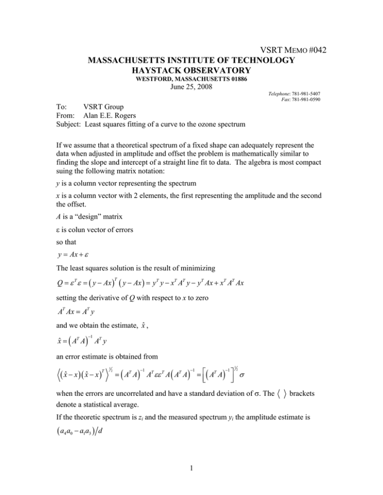
VSRT MEMO #042
MASSACHUSETTS INSTITUTE OF TECHNOLOGY
HAYSTACK OBSERVATORY
WESTFORD, MASSACHUSETTS 01886
June 25, 2008
Telephone: 781-981-5407
Fax: 781-981-0590
To:
VSRT Group
From: Alan E.E. Rogers
Subject: Least squares fitting of a curve to the ozone spectrum
If we assume that a theoretical spectrum of a fixed shape can adequately represent the
data when adjusted in amplitude and offset the problem is mathematically similar to
finding the slope and intercept of a straight line fit to data. The algebra is most compact
suing the following matrix notation:
y is a column vector representing the spectrum
x is a column vector with 2 elements, the first representing the amplitude and the second
the offset.
A is a “design” matrix
ε is colun vector of errors
so that
y = Ax + ε
The least squares solution is the result of minimizing
Q = ε T ε = ( y − Ax )
T
( y − Ax ) = yT y − xT AT y − yT Ax + xT AT Ax
setting the derivative of Q with respect to x to zero
AT Ax = AT y
and we obtain the estimate, x̂ ,
xˆ = ( AT A ) AT y
−1
an error estimate is obtained from
( xˆ − x )( xˆ − x )
T
1
−1
−1
−1 2
= ( AT A ) AT εε T A ( AT A ) = ⎡⎢( AT A ) ⎤⎥ σ
⎣
⎦
1
2
when the errors are uncorrelated and have a standard deviation of σ. The
brackets
denote a statistical average.
If the theoretic spectrum is zi and the measured spectrum yi the amplitude estimate is
( a4 a0 − a1a3 )
d
1
N −1
where a4 = ∑ zi yi
i =0
a0 = N
a1 = ∑ zi
a3 = ∑ yi
d = a0 a2 − a12
The error estimate in amplitude
d 2σ
−1
Reference:
Bevington, P.R., Robinson, D.K., “Data reduction and error analysis the physical
sciences,” McGraw-Hill, 1992.
2