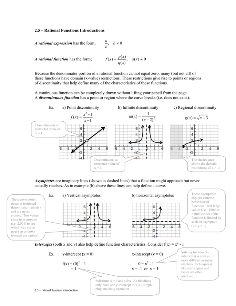
2.5 – Rational Functions Introductions
A rational expression has the form;
a
, b≠0
b
A rational function has the form;
f ( x) =
p( x)
, q( x) ≠ 0
q ( x)
Because the denominator portion of a rational function cannot equal zero, many (but not all) of
these functions have domain (x-value) restrictions. These restrictions give rise to points or regions
of discontinuity that help define many of the characteristics of these functions.
A continuous function can be completely drawn without lifting your pencil from the page.
A discontinuous function has a point or region where the curve breaks (i.e. does not exist).
Ex.
a) Point discontinuity
f ( x) =
2
x −1
x −1
b) Infinite discontinuity
1
m( x ) =
( x − 2)2
c) Regional discontinuity
g ( x) = x + 3
Discontinuous at
restricted value of
x=1
Discontinuous at
restricted value of
x=2
The shaded area
shows the domain
restrictions of x ≥ -3
Asymptotes are imaginary lines (shown as dashed lines) that a function might approach but never
actually reaches. As in example (b) above these lines can help define a curve.
These asymptotes
occur at restricted
denominator value(s)
and are never
crossed. Test values
close to asymptote
(i.e. 2.001) to see
which way curve
goes (up or down
towards asymptote)
Ex.
a) Vertical asymptotes
These asymptotes
explore extreme
behaviour of
functions. Test large
values (i.e. -1000 or
+1000) to see if the
function is limited by
such an asymptote
(i.e. y = 1)
b) horizontal asymptotes
Intercepts (both x and y) also help define function characteristics. Consider f(x) = x2 - 1
Ex.
y-intercept (x = 0)
x-intercept (y = 0)
f(x) = (0)2 – 1
=1
0 = x2 - 1
x = -1 or x = 1
2.5 – rational function introduction
Substitute x = 0 and solve. As functions
only have one y-intercept this is a simple
plug and chug operation
Solving for zero (xintercepts) is always
more difficult as many
algebraic technique(s)
like rearranging and
factor are often
involved.
Although there are several different types of rational functions, we will be studying and
transforming two main types. The simplest forms of these two functions are shown below.
Ex.
a) Reciprocal Linear Functions
f ( x) =
b) Reciprocal Quadratic Functions
1
x
f ( x) =
1
x2
Use the graphing calculator to graph the following functions and complete the table to gain
insight into some rational functions and their characteristics. You will need to copy the chart into
your own notes so that you can fit in adequately sized graphs.
Function
Vertical
asymptotes
Sketch
Horizontal
Asymptotes
Intercepts
(discontinuity)
(extreme
behaviour)
y
x
n/a
y=0
½
n/a
1
x−2
1
f ( x) = − 2
x
1
f ( x) =
( x − 2) 2
1
f ( x) =
( x + 2) 2
f ( x) =
f ( x) =
1
( x − 2)
f ( x) =
1
2
( x + 2)
2
1
0.5
0
-10
x
x−2
x2
f ( x) =
x − 2)
f ( x) =
f ( x) =
x
( x + 2)( x − 1)
2.5 – rational function introduction
-5
-0.5
0
5
10
2.5 - Sketching Practice Sheet
2.5 – rational function introduction