David Spain CS7641 Assignment #1 Supervised Learning Report
advertisement
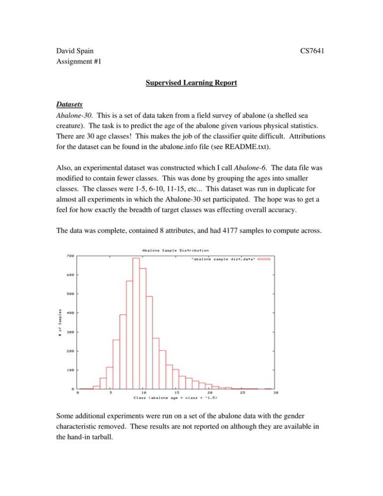
David Spain Assignment #1 CS7641 Supervised Learning Report Datasets Abalone­30. This is a set of data taken from a field survey of abalone (a shelled sea creature). The task is to predict the age of the abalone given various physical statistics. There are 30 age classes! This makes the job of the classifier quite difficult. Attributions for the dataset can be found in the abalone.info file (see README.txt). Also, an experimental dataset was constructed which I call Abalone­6. The data file was modified to contain fewer classes. This was done by grouping the ages into smaller classes. The classes were 1­5, 6­10, 11­15, etc... This dataset was run in duplicate for almost all experiments in which the Abalone­30 set participated. The hope was to get a feel for how exactly the breadth of target classes was effecting overall accuracy. The data was complete, contained 8 attributes, and had 4177 samples to compute across. Some additional experiments were run on a set of the abalone data with the gender characteristic removed. These results are not reported on although they are available in the hand­in tarball. Vehicle. The dataset was originally purposed to examine whether 3D objects could be distinguished from a 2D image representation. The images have been processed and values for their feature attributes created by the HIPS system (see vehicle.info file). There are four cars which we are attempting to recognize: Opel, Saab, Bus, Van. There are 18 feature attributes and 946 data points in the set. Why are these interesting datasets? The datasets were interesting both for their practical implications and for the results they gave when supervised learning techniques were applied to them. Abalone have gone through a period of significant decline in recent years due to both natural and unnatural environmental pressures (reintroduction of sea otters, loss of habitat). If techniques to determine age could be used that did not require killing the abalone in order to sample the population, this would be beneficial. Here the abalone were destroyed to create an accurate age profile. The vehicle dataset is of practical interest to many vision problems. For example, a technology like this one could be quite useful in creating an agent who drives a car. This is already an idea that has quite an active (or at least well publicized) following. With respect to machine learning, why are these interesting datasets? The abalone dataset is of interest in many ways because it is so resistant to good performance under machine learning techniques. None of the supervised learning techniques that are presented here achieve particularly good results (though they are improved for the Abalone­6 dataset). While it is somewhat beyond the scope of the assignment to pursue HOW exactly to make a dataset like this perform well, I did get a stronger intuition for why the dataset does not lend itself to be “cracked” by ML methods (the large # of classes and the highly clustered data that does not split easily onto a particular class). The vehicle dataset is generally of interest as an example of a vision problem. One thing that I do, in retrospect, think that the dataset suffers from is a lack of examples. There are 18 attributes, but only a 1000 examples. The curse of dimensionality makes this a sparse enough sampling of the space that it is difficult to get highly accurate results. Decision Trees prune state|confidence|# leaves|tree size|train %|test %|train time|test time # Abalone-30 pruned 0.125 996 pruned 0.25 1183 pruned 0.5 1215 unpruned --1301 # Abalone-6 pruned 0.125 pruned 0.25 pruned 0.5 unpruned --# Vehicle pruned pruned pruned unpruned 0.125 0.25 0.5 --- 180 247 338 397 75 98 98 104 1944 2312 2374 2540 71.0558 75.7242 76.2988 77.0409 % % % % 21.786 21.1635 20.8762 20.5889 % % % % 3.93 1.84 4.02 1.57 0.32 0.16 0.35 0.16 347 477 652 762 79.6026 81.5897 83.457 83.9598 % % % % 68.7575 67.321 66.8422 66.6507 % % % % 1.68 0.73 1.53 0.62 0.18 0.05 0.09 0.05 149 195 195 207 94.0898 96.9267 96.9267 97.1631 % % % % 72.4586 72.4586 72.695 72.8132 % % % % 0.55 0.9 0.51 0.77 0.04 0.24 0.04 0.03 confusion matrix for Abalone-30, confidence 0.125 0 0 1 0 0 0 0 0 0 0 0 0 0 0 0 1 0 0 0 0 0 0 0 0 2 0 0 12 1 0 0 0 0 0 0 0 1 0 3 28 16 8 1 0 0 0 0 0 0 0 1 23 33 36 14 3 4 1 0 0 0 0 0 10 28 87 87 25 9 7 2 2 0 0 0 6 13 85 113 89 39 25 10 5 0 0 0 2 10 32 87 154 138 78 31 20 0 0 0 0 2 22 44 132 191 139 83 36 0 0 0 0 0 10 31 79 140 146 102 37 0 0 0 0 0 3 10 47 87 123 108 45 0 0 0 0 0 2 8 24 52 56 67 16 0 0 0 0 0 4 4 9 28 48 47 10 0 0 0 0 0 1 3 5 17 19 23 13 0 0 0 0 0 0 1 7 16 19 19 11 (a portion of it) 0 0 0 0 0 0 0 0 0 0 0 0 0 0 0 0 0 0 0 0 0 0 0 0 0 0 0 0 0 2 2 2 1 1 0 9 4 1 0 2 16 6 9 4 5 41 20 12 5 4 32 6 11 3 8 19 8 6 4 3 17 17 4 10 2 16 5 11 5 3 9 6 2 2 5 0 0 0 0 0 0 0 0 0 2 2 0 1 1 0 0 0 0 0 0 0 0 0 0 3 1 2 1 3 2 0 0 0 0 0 0 0 0 0 2 1 0 1 0 4 0 0 0 0 0 0 0 0 0 0 0 0 0 0 0 There are several features of note that are evident in the results for decision trees. First, the pruning actually improves accuracy slightly on the test set for Abalone* and has a negligible impact on the Vehicle dataset. In the case, of the abalone test sets, I believe that is slight improvement is basically the result of undoing some of the overfitting that the decision tree has done in this case. It is interesting that being fairly aggressive in pruning is yielding these results. This makes sense in the context of the abalone dataset. The measurements of the physical properties of the abalone should, intuitively, be fairly overlapped. I say this because they basically grow slowly for thirty years without particularly much boom and bust to their food supply. With this as a background, it makes sense that a decision tree might overfit the data somewhat given that the data are not easily separable. The “abalone.info” file gives some statistics and citations that back this observation. Second, it is also easy to observe that the training vs testing times follow what we would expect for an eager learner. The training phase takes significantly more time than the testing phase. Finally, the low success rate for Abalone­30 is interesting (approx 20%). There are two potential interpretations for this data that I can come up with. The fact that there are 30 classes makes the problem of identifying which class a given abalone belongs to very difficult. This is akin to the example Charles gave in class about a decision tree not dealing well when there is too much granularity in the classes to choose from (ex: date/time could be a problem attribute!). Alternately, we can look at the confusion matrix for this problem. Doing so allows us to realize that although the learner does not guess the correct answer all that often, neither is he off by more than a couple years particularly frequently. I did not calculate the error rate if you allowed the learner to count successes as anything +or­ a couple years, though the excerpted portion of the matrix shows that the correctness rate would improve significantly! The significantly increased success of the Abalone­6 dataset captures some of this idea. Though with it's static borders, it still retains some of the bias for failure on edge ages (ex: classes 1­5,6­10, edge ages 5 & 6). Note regarding the confusion matrix: The correct guesses fall on the diagonal. Incorrect guesses are placed off the diagonal. Neural Networks (mislabelled! The above is for Abalone­30) The experiments that I ran regarding neural networks were quite interesting in many ways. In the three graphs above, I ran the datasets with several different learning rates and momentums. The results you can see in the left hand portions of the graph appear quite different until the scale of the y axis is considered. While the results do see to be on different trajectories (some up, some down), they are clustered within a percentage or two of each other. The differing behaviors under different learning rates with runs of differing epoch lengths, does point out that the hypersurface representing the “true” concept in these datasets likely has plenty of complexity to explore. It would be interesting to re­run these results and plot the changes in the network weights to get an idea of the vectors that are being generated during backpropagation. This is beyond what I could accomplish here. It is also interesting to note that there is one common feature to the runs of 5000 epochs and beyond. It appears that the process of overfitting the network to the idiosyncracies of the dataset has begun. In the two graphs below (one from vehicles, the other from abalone), we can see that the training error and test errors are beginning to diverge. Finally, the times for the neural networks epitomized eager learners. As an example, an Abalone­30 run with 10,000 epochs took 5.36 hours of cpu time to train and 1.01 seconds to test. (mislabelled, this is Abalone­30). Note that the test accuracy is declining while the training accuracy is still increasing. Boosting prune state|boost iterations|dtree pruning confidence|train %|test % # Abalone-30 pruned 10 pruned 10 pruned 10 unpruned 10 pruned 20 pruned 20 pruned 20 unpruned 20 pruned 40 pruned 40 pruned 40 unpruned 40 0.125 0.25 0.5 --0.125 0.25 0.5 --0.125 0.25 0.5 --- 99.7606 99.9521 100 100 100 100 100 100 100 100 100 100 % % % % % % % % % % % % 21.786 21.7381 21.6184 21.4029 21.8339 21.8817 22.193 21.786 22.5042 22.2648 21.6902 22.169 % % % % % % % % % % % % # Abalone-6 pruned 10 pruned 10 pruned 10 unpruned 10 pruned 20 pruned 20 pruned 20 unpruned 20 pruned 40 pruned 40 pruned 40 unpruned 40 0.125 0.25 0.5 --0.125 0.25 0.5 --0.125 0.25 0.5 --- 100 100 100 100 100 100 100 100 100 100 100 100 % % % % % % % % % % % % 65.1664 65.1185 64.1848 63.7299 66.6028 66.2677 64.6636 65.2382 66.3155 66.7704 66.6507 65.9804 % % % % % % % % % % % % # Vehicle pruned 10 pruned 10 pruned 10 unpruned 10 pruned 20 pruned 20 pruned 20 unpruned 20 pruned 40 pruned 40 pruned 40 unpruned 40 0.125 0.25 0.5 --0.125 0.25 0.5 --0.125 0.25 0.5 --- 100 100 100 100 100 100 100 100 100 100 100 100 % % % % % % % % % % % % 77.896 76.2411 78.6052 77.5414 78.3688 76.9504 78.8416 78.6052 78.3688 77.896 79.078 78.7234 % % % % % % % % % % % % Boosting was performed using the same decision tree code that was used in the Decision Tree section of this report. It is interesting that the Abalone­30 & ­6 datasets actually showed slight declines in performance under boosting. This was the case regardless of the aggressiveness or lack thereof that I utilized in the decision tree pruning! While the difference was no more than a percent or two, it appears that the nature of the abalone set makes it resistant to getting better results via this technique given the data provided. Per the abalone.info file the data examples are “highly­overlapped”. Though, theoretically boosting should be lowering the bounds on the error, in practice it still requires a dataset that is has more distinguishing features. The vehicle dataset did show improvement (5­7%). This is the trend that I expected, given the boosting technique. One other interesting observation about boosting is that it appears to take on the run time profile of the algorithm being boosted. Also, the time to build the model varies close to linearly in the number of boosting iterations that are used. For example, running the vehicle dataset through 10, 20, and 40 iterations with pruning confidence set to 0.125 took 25, 60, 130 seconds. k­NN At first glance it is surprising that kNN works so much better for the abalone set than the other machine learning algorithms have (not that it is great). It shows about a 5% performance improvement over the other techniques. Why? The reason that I would guess that this works is largely due to the distribution of samples from the sample data. In the distribution graph of the abalone ages (early in the report), we can see that about 50% of the abalone samples are between ages 6­11. With this density, if I am looking at an abalone of a particular age, it is likely that my neighbors will actually be of my age or off by no more than 1 or 2 years. (the training line is at 100% all the way across) The vehicle graphs above show a small gain for the kNN algorithm when using the weighted sampling. This probably works because the attributes that are in use for making our class prediction are all contributing to prediction correctness. In an attribute landscape where some attributes are not providing relevant information to the problem at hand, we could expect that some of the “nearest neighbors” might be arbitrary matches on non­relevant attributes. This would corrupt our results. Alternately, one or more of the attributes might not be especially relevant, but due to the small size of the dataset (1000 data points) the “nearest neighbor” chance collisions may not have occurred. This latter hypothesis seems unlikely since the attributes were hand­selected by a domain expert for exactly the task we are using them for. Support Vector Machines Kernel|exponent or gamma|train %|test %|train time|test time #Abalone-6 poly 1 poly 2 poly 3 RBF 0.01 RBF 0.5 RBF 1.0 68.9729 69.4039 70.3376 60.8331 68.2068 68.9251 % % % % % % 68.566 69.1884 69.6912 60.8331 67.9435 68.5899 % % % % % % 3.89 96.45 364.85 142.12 159.16 99.69 0.08 8.02 26.67 16.22 27.12 15.22 # Abalone-30 poly 1 poly 2 poly 3 RBF 0.01 RBF 0.5 RBF 1.0 25.5207 26.8853 27.3881 20.3735 26.2868 26.9332 % % % % % % 25.2334 26.1192 26.4065 20.3495 25.4489 25.808 % % % % % % 27.57 143.91 204.72 80.79 95.81 70.75 0.87 100.83 191.83 119.18 223.75 114.2 # Vehicle poly 1 poly 2 poly 3 RBF 0.01 RBF 0.5 RBF 1.0 76.2411 84.5154 89.0071 46.2175 77.6596 81.5603 % % % % % % 74.3499 80.3783 83.8061 40.0709 74.8227 75.5319 % % % % % % 0.51 1.79 2.14 3.19 1.39 2.22 0.04 0.83 0.71 3.84 1.26 2.65 For these experiments I used two different kinds of kernels: a polynomial kernel with a varying exponent and a Radial Basis Function kernel varying gamma. I was unable to find documentation relating to what exactly gamma was despite an extensive web search. This was frustrating, because the change in gamma relates to one of the most dramatic improvements shown by any of the supervised learning algorithms. In the vehicle set, changing gamma from 0.01 to 0.5 produced a 34% improvement in the test set results (using cross­validation as always). I assume that this parameter may relate somehow the std deviation size being used at each of the different RBF nodes, but I don't know! The polynomial function support vector functions also showed improvements as the exponent argument was increased. This makes sense as the exponent should allow more freedom in how to create the maximal margin between the various classes. Notably though, utilizing a high exponent increases both training and testing times significantly!
