CSC 446 Notes: Lecture 17
Typed by Ian Perera
April 10, 2012
1
Hidden Markov Models
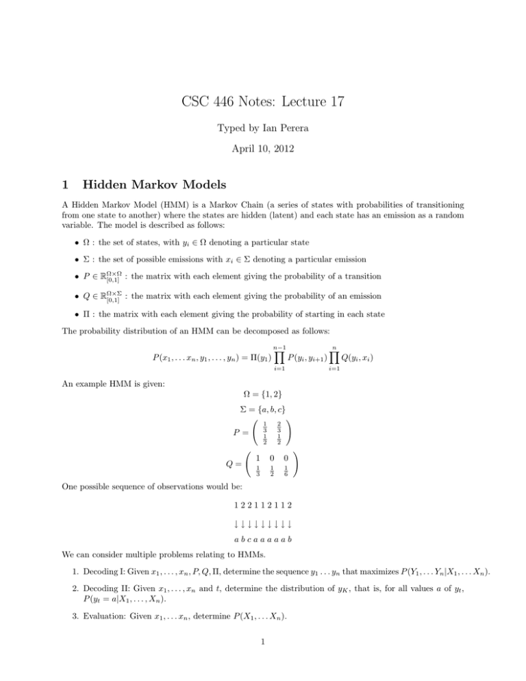
A Hidden Markov Model (HMM) is a Markov Chain (a series of states with probabilities of transitioning
from one state to another) where the states are hidden (latent) and each state has an emission as a random
variable. The model is described as follows:
• Ω : the set of states, with yi ∈ Ω denoting a particular state
• Σ : the set of possible emissions with xi ∈ Σ denoting a particular emission
• P ∈ RΩ×Ω
[0,1] : the matrix with each element giving the probability of a transition
• Q ∈ RΩ×Σ
[0,1] : the matrix with each element giving the probability of an emission
• Π : the matrix with each element giving the probability of starting in each state
The probability distribution of an HMM can be decomposed as follows:
P (x1 , . . . xn , y1 , . . . , yn ) = Π(y1 )
n−1
Y
P (yi , yi+1 )
n
Y
Q(yi , xi )
i=1
i=1
An example HMM is given:
Ω = {1, 2}
Σ = {a, b, c}
1
3
1
2
P =
Q=
2
3
1
2
!
1
0
0
1
3
1
2
1
6
!
One possible sequence of observations would be:
122112112
↓↓↓↓↓↓↓↓↓
abcaaaaab
We can consider multiple problems relating to HMMs.
1. Decoding I: Given x1 , . . . , xn , P, Q, Π, determine the sequence y1 . . . yn that maximizes P (Y1 , . . . Yn |X1 , . . . Xn ).
2. Decoding II: Given x1 , . . . , xn and t, determine the distribution of yK , that is, for all values a of yt ,
P (yt = a|X1 , . . . , Xn ).
3. Evaluation: Given x1 , . . . xn , determine P (X1 , . . . Xn ).
1
(1)
(1)
(k)
(k)
4. Learning: Given a sequence of observations, x1 , . . . xn , . . . x1 , . . . xn , learn P, Q, Π that maximize
the likelihood of the observed data.
We define two functions, α and β.
αt (a) := P (X1 = x̂1 , . . . , Xt = x̂t , Yt = a)
β t (a) := P (Xt+1 = x̂t+1 , . . . , Xn = x̂n , Yt = a)
which are also recursively defined as follows:
X
αt+1 (a) =
αt (c)P (c, a)Q(a, x̂t+1 )
c∈Ω
X
β t−1 (a) =
Q(c, x̂t )β t (c)P (a, c)
c∈Ω
We return to the Decoding II problem. Given x1 , . . . , xn and t, determine the distribution of YK , that is,
for all values a of Yt , P (Yt = a|X1 , . . . , Xn ). To do this, we rewrite the equation as follows:
P (yt = a|X1 , . . . , Xn ) =
P (X1 , . . . , Xn , Yt = a)
.
P (X1 , . . . , Xn )
However, we need to calculate P (X1 , . . . , Xn ). We can do this using either α or β.
X
P (X1 , . . . , Xn ) =
αn (a)
a∈Ω
=
X
β 1 (a)Π(a)Q(a, x̂1 )
a∈Ω
The Decoding I problem can be solved with Dynamic Programming. (Given x1 , . . . , xn , P, Q, Π, determine
the sequence y1 . . . yn that maximizes P (Y1 , . . . Yn |X1 , . . . Xn ).) We can fill in a table with the following
values:
T [t, a] = max P (y1 , . . . yt |X1 , . . . Xt )
y1 ...yt ,yt =a
which means that each value is the probability of the most likely sequence at time t with the last emission
being a. This can be computed using earlier values with the following formula:
T [t + 1, a] = max T [t, c]P (c, a)Q(a, x̂t+1 )
c∈Ω
To compute the most likely sequence, we simply solve
max T [n, a]
a∈Ω
The learning problem can be solved using EM. Given the number of internal states, and x1 , . . . xn , we want
to figure out P , Q, and Π. In the E step, we want to compute an expectation over hidden variables:
X
P (X, Y |θ)
L(θ, q) =
q(y|x) log
q(Y |X)
y
For HMM’s, the number of possible hidden state sequences is exponential, so we use dynamic programming
to compute expected counts of individual transitions and emissions:
P (a, b) ∝
Q(a, b) ∝
n−1
X
i=1
n
X
q(Yi = a, Yi−1 = b|X1 . . . Xn )
(1)
q(Yi = a|X1 . . . Xn )I(X = w)
(2)
i=1
The new P is defined as:
P new (a, b) ∝
n−1
X
αi (a)P old (a, b)β i+1 Qold (b, x̂i+1 )
i=1
2