2
Convex Hulls
2.1
Definitions
Convexity is the key to understanding and simplifying geometry, and the convex hull
plays a role in geometry akin to the “sorted order” for a collection of numbers.
So what is a convex set ? The easiest way to define it is in Euclidean space, or more
generally in a vector space over the reals.
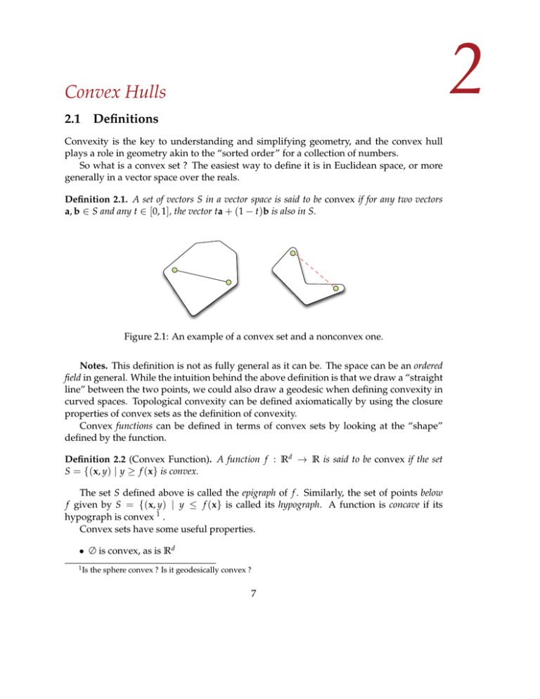
Definition 2.1. A set of vectors S in a vector space is said to be convex if for any two vectors
a, b 2 S and any t 2 [0, 1], the vector ta + (1 t)b is also in S.
Figure 2.1: An example of a convex set and a nonconvex one.
Notes. This definition is not as fully general as it can be. The space can be an ordered
field in general. While the intuition behind the above definition is that we draw a “straight
line” between the two points, we could also draw a geodesic when defining convexity in
curved spaces. Topological convexity can be defined axiomatically by using the closure
properties of convex sets as the definition of convexity.
Convex functions can be defined in terms of convex sets by looking at the “shape”
defined by the function.
Definition 2.2 (Convex Function). A function f : R d ! R is said to be convex if the set
S = {(x, y) | y
f (x} is convex.
The set S defined above is called the epigraph of f . Similarly, the set of points below
f given by S = {(x, y) | y  f (x} is called its hypograph. A function is concave if its
hypograph is convex 1 .
Convex sets have some useful properties.
• ∆ is convex, as is R d
1 Is
the sphere convex ? Is it geodesically convex ?
7
8
CHAPTER 2. CONVEX HULLS
S = {(x, y) | y
x2 }
S = {(x, y) | y 
6
0
6
p
0
x}
6
Figure 2.2: Convex and concave functions
• The intersection of any two convex sets is convex.
• In general, the union of two convex sets is not convex
If we have two points a1 , a2 , the set S = {ta1 + (1 t)a2 | 0  t  1} is the straight
line connecting the two points. A more general way of writing this is S = {l1 a1 + l2 a2 |
l1 + l2 = 1, li
0}. For any fixed li satisfying the above constraints, the combination
Âi li pi is called the convex combination.
This allows us to generalize the notion to more than two points.
Definition 2.3 (Convex Hull). The convex hull of a set of points is the set S = {Âi li pi |
 li = 1, li 0}. This is also called a convex polytope.
For two points, we’ve seen that this is the straight line connecting the points. For three
points, we get the triangle with the three points as corners.
The convex hull can also be defined as the smallest convex set containing the points,
where “smallest” here means that there is no other set contained in the first that also
contains the points. This alternate definition is useful if we wish to define convexity in
more general spaces.
H-representation. The representation of a convex set described above is often called the
V-representation, since it’s expressed in terms of vertices of the resulting convex polytope.
There is an alternate view of a convex set that’s equally important.
A hyperplane is described as S = {x | ha, xi = b}, where a is a normal to the plane. A
halfspace (one side of the hyperplane) can be described as ha, xi  b. Note that a halfspace
is convex !
So let’s stack up a number of halfspaces and compute their intersection. Since each
halfspace is described by the pair ai , bi , we can put them all together in the matrix equation
Ax  b
2.2. COMPUTING PLANAR CONVEX HULLS
9
The space defined by these inequalities is called a polyhedron. We’ll say that the polyhedron is bounded if it can be contained in some bounded region.
A deep result in the theory of polytopes says that bounded polyhedra and polytopes are
the same thing. Specifically,
Theorem 2.1 (Finite basis[4]). A set S is a polytope iff it is a bounded polyhedron.
One way to interpret this is as saying that any bounded polyhedron in a finite-dimensional
space can be generated as the convex hull of a finite set of points.
The extension to unbounded polyhedra is not very different. The equivalent characterization result says that a general polyhedron can always be written as the sum of a
polytope and a cone2
2.2
Computing planar convex hulls
Suppose we are a given a collection of points, and wish to compute the convex hull. For
now, let’s say that we’re in the plane. Here, the boundary of the hull consists of line
segments connecting points, and so the complexity of the boundary is twice the number
of points on it.
Jarvis March. The simplest algorithm to compute the convex hull is often called the giftwrapping algorithm, or the Jarvis march[2]. Imagine taking a thread and winding it around
a point that is sure to be on the hull. Then as you wrap it around the point set, it will pick
off the convex hull vertices one by one.
Algorithm 1 The Jarvis March
Find the leftmost point p1 . Call it c1 . Set c0 to be a point vertically above c1
for i = 2 . . . h do
Find point p 2 P such that ci p has smallest slope greater than ci 1 ci .
Set ci = p.
end for
This algorithm runs in time O(nh) if h is the size of the convex hull. And if you don’t
know h, just run it till you return to c1 . It works because c1 is guaranteed to be on the hull,
and at all times we are constructing a set of lines that completely contain the point set on
one side.
2 I’ll
explain this later
10
CHAPTER 2. CONVEX HULLS
Andrew’s Algorithm The above algorithm is fine if h is small. But since h can be n (think
of points on a circle), the worst-case running time is O(n2 ). Can we do better ?
The next algorithm runs in time O(n log n) regardless of the size of the hull. The idea
is to preprocess the input and use the order to help decide which points to pick.
Algorithm 2 Andrew’s algorithm
Sort all the points by x-coordinate. Renumber so that p1 is the left-most point.
/* Now compute the upper hull */
Push p1 , p2 , p3 onto a stack.
while there are unpushed points do
Take top three points c 2 , c 1 , c0 on stack.
if they form a left turn then
Push c 2 , c0 back onto stack./* deleted c 1 */
else
Push next point from sorted list onto stack
end if
end while
Output contents of stack in order
/* repeat backwards for lower hull */
The sorting takes O(n log n) time, and the rest of the procedure only takes linear time
! This is easy to see by an indirect argument. Notice that each point is touched at most
twice. Once when it’s pushed onto the stack, and once if it’s removed later on. This
implies that the total amount of work involved is linear in the input.
Chan’s algorithm Both of the above algorithms work well under certain circumstances
and are inefficient under others. Can we design an algorithm that is optimal for all inputs
?
This next algorithm due to Timothy Chan[1] is extremely simple. It combines the
above two methods in a clever way in order to achieve a bound of O(n log h) for computing an h-sized convex hull of n points.
There are two key ideas. Firstly, we guess the size of the convex hull: call this guess
m. Later, we will see how to make this guess “correct”. A second insight is that in the
Jarvis march, finding the next point of the hull is a lot easier if the set you’re searching
over already has a convex hull, because you can do a binary search over the boundary of
the hull instead of examining all the points.
We first partition the points arbitrarily into dn/me groups of size m. In each group, we
use Andrew’s algorithm to compute a convex hull. The overall running time of this step
is O((n/m) · m log m = n log m).
2.2. COMPUTING PLANAR CONVEX HULLS
11
Now we run the Jarvis march on the collection of hulls. At each step, we need to
pick a point such that the resulting slope is as small as possible relative to our current
direction. For each convex hull, this point can be found using binary search in O(log m)
time (since each hull has size at most m). The overall running time of each iteration is
therefore O(n/m · log m), and the total running time is O(n log m) again (since we run it
for m steps).
Algorithm 3 FindHull(P, m)
Partition P into n/m groups Pi
for i = 1 . . . n/m do
Hi = ConvexHull( Pi )
end for
Run Jarvis march on {Hi } for m steps
if we get a complete hull then
return success
else
return fail
end if
But how do we make our guess ? Notice that if our guess m is less than the true hull
size h, then at some point we will have picked m points to be on the hull, but we would
not have reached our starting point. So it’s possible to detect if m  h. However, we don’t
want to overshoot h by too much, because the running time might become too large.
Since the overall running time for a guess m is O(n log m), we merely need to make
sure that log m = O(log h). This can be achieved by repeatedly guessing values of log m,
and doubling our guess each time. If we overshoot, then log m  2 log h.
Algorithm 4 Chan’s algorithm
i=0
i
while FindHull(P, 22 ) fails do
i
i+1
end while
i
So we set log m = 2, 4, 8, . . . , log h, which corresponds to setting m = 22 , 0  i 
12
CHAPTER 2. CONVEX HULLS
log log h. The overall running time is then
log log h
T (n) =
Â
n log 22
i
i =0
log log h
=n
Â
2i
i =0
log log h+1
 n2
= n log h
2.3
Higher Dimensions
The above algorithm generalizes to three dimensions, and there are other techniques you
can apply as well. When things get to high dimensions, the problem gets harder.
First of all, let’s talk about the representation. In d dimensions, a polytope admits
facets of all dimensions: vertices are 0-dimensional, lines are 1-dimensional, and so on.
The convex hull is then written as the set of all the facets and their adjacency relationships.
Since all faces are at most d-dimensional, there’s a clear O(nd ) upper bound on the
total complexity of all the facets. But this is no good even in two dimensions.
The Upper Bound Theorem due to McMullen[3] states that the total complexity of the
convex hull of n points in d dimensions is O(nbd/2c ). The proof is quite complicated and
involves the idea of a shelling of a polytope.
But we can ask a simpler question: how many vertices can a polytope defined by n
inequalities have ? Here, Seidel gave a beautiful two-line proof (the proof is in fact in the
abstract of his paper[5]).
The idea is as follows. Each vertex of the polytope is defined by the intersection of d
halfplanes. In particular, each vertex has d edges (1-faces) emanating from it. Fix some
direction so that all vertices are at different “heights”. Now each vertex has d edges emanating from it, and at least dd/2e of these edges point “up” or “down”. These edges will
define a face of the polytope (why?). Therefore, the total number of vertices is at most the
sum of the number of facets of dimension at least dd/2e. There can be at most (d n k) facets
of dimension k. Summing up, we get the desired bound.
Lower bounds. The above bound is tight. In fact, McMullen showed a stronger result;
namely that the complexity of a polytope with n vertices in d dimensions is at most the
complexity of the cyclic polytope.
The cyclic polytope is constructed as follows. Define the moment curve f (t) : R ! R d
as the curve
f (t) = (t, t2 , . . . , td )
2.4. THE DATA CONNECTION
13
Take any n points on this curve and compute their convex hull. This is the cyclic
polytope. It has the property that any set of bd/2c points define a face. Also note that
this is the dual of the bound we are looking for: it lower bounds the complexity of the
number of faces of a polytope on n vertices, rather than bounding the number of vertices
of a polyhedron defined by n inequalities. We’ll talk about geometric duality a little later.
2.4
The Data Connection
The convex hull is a basic data structure that we use in computational geometry. It’s also
a way to reduce data size. Consider the problem of finding the diameter of a point set:
the maximum distance between any two points in the set. A little thought reveals that
this distance must be achieved by two points on the boundary of the convex hull and that
these two points must be on “opposite sides” of the hull. This is the basis for the rotating
calipers method[6].
Consider now the problem of classification. In (linear) binary classification, you’re
given two sets of points and must find a hyperplane that separates them by as large a
margin as possible. Again, a little thought reveals that this is the problem of finding the
closest pair of points between two polytopes: one being the convex hull of one set, the
other being the convex hull of the other. This insight leads to many algorithms for solving
the binary classification problem.
Figure 2.3: Classification and convex hulls
2.5
After Notes
The curse of dimensionality. The bound for the d-dimensional convex hull is our first
encounter with the curse of dimensionality. This is the principle that many geometric structures of interest grow exponentially with the dimension, and here we see this to be true for
the complexity of the convex hull.
What this means is that if we want to retain the benefits of the convex hull in high
dimensions, we will need to find a way to avoid computing the convex hull explicitly.
14
CHAPTER 2. CONVEX HULLS
Convex, Affine, Linear and Conic Combinations. Convex combinations are only one of
four different ways to combine points. Depending on the conditions we place on the li ,
we get different types of combinations. These can be summarized in a convenient table.
li
0
True
False
 li = 1
True
False
Convex Conic
Affine Linear
Table 2.1: Different combinations of points. In each case, we compute the set S = {Â li pi }
Exercises.
1. Andrew’s algorithm requires points to be sorted, and this is the source of the O(n log n)
bound. Maybe we could do better without a sorted order. Suppose we had a simple
polygon, and we ran the algorithm in the order of the points on the boundary of the
polygon. Would it work ?
2. We are given three points in R3 . Describe their convex hull, affine hull, conic hull,
and linear hull. Remember that the x-hull is formed by taking all possible x-combinations
of the points.
3. Describe a divide-and-conquer-based strategy to compute the convex hull of n
points in the plane in O(n log n) time.
4. How does the problem of finding a maximum margin classifier separating two sets
of points reduce to the problem of finding the closest pair between two polytopes ? You
may explain your answer in the plane.
Bibliography
[1] T. Chan. Optimal output-sensitive convex hull algorithms in two and three dimensions. Discrete & Computational Geometry, 16(4):361–368, 1996.
[2] R. Jarvis. On the identification of the convex hull of a finite set of points in the plane.
Information Processing Letters, 2(1):18–21, 1973.
[3] P. McMullen. The maximum numbers of faces of a convex polytope. Mathematika,
17:179–184.
[4] A. Schrijver. Theory of linear and integer programming. Wiley, 1998.
[5] R. Seidel. The upper bound theorem for polytopes: an easy proof of its asymptotic
version. Computational Geometry, 5(2):115–116, 1995.
[6] G. Toussaint. Solving geometric problems with the rotating calipers. In Proc. IEEE
Melecon, volume 83, page A10, 1983.
15