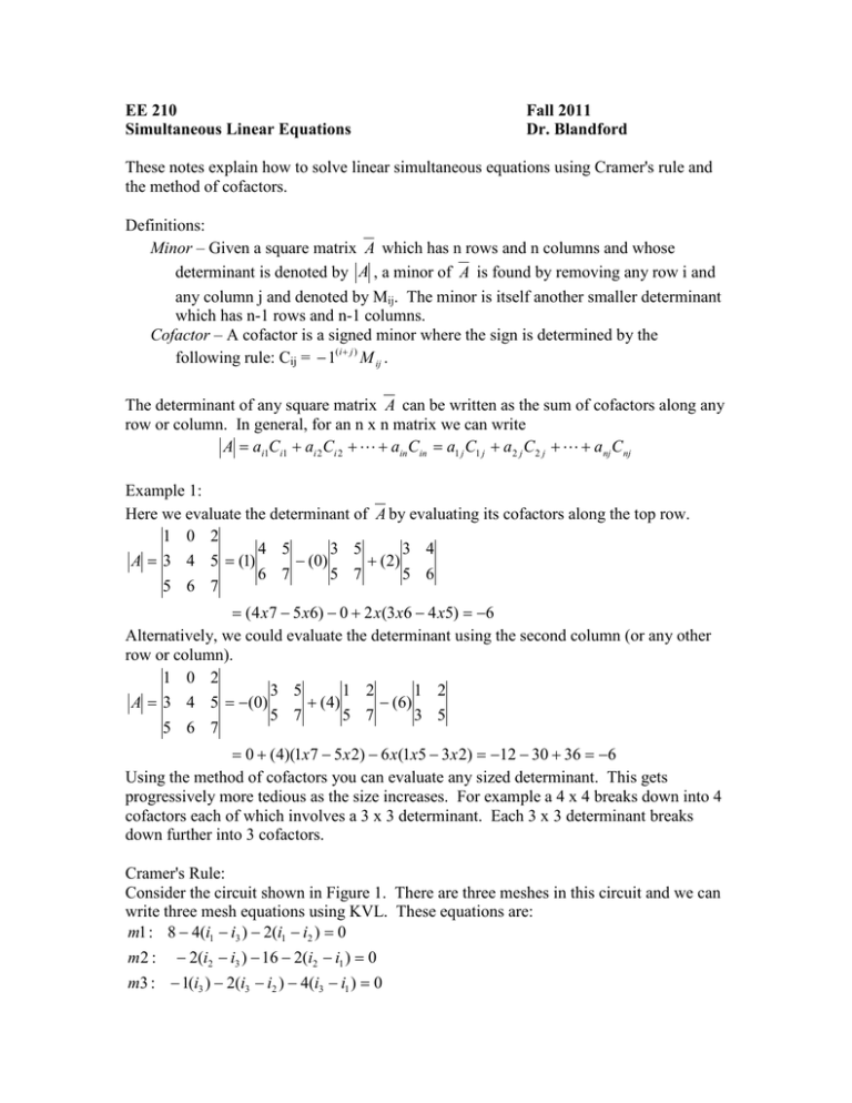
EE 210
Simultaneous Linear Equations
Fall 2011
Dr. Blandford
These notes explain how to solve linear simultaneous equations using Cramer's rule and
the method of cofactors.
Definitions:
Minor – Given a square matrix A which has n rows and n columns and whose
determinant is denoted by A , a minor of A is found by removing any row i and
any column j and denoted by Mij. The minor is itself another smaller determinant
which has n-1 rows and n-1 columns.
Cofactor – A cofactor is a signed minor where the sign is determined by the
following rule: Cij = − 1(i + j ) M ij .
The determinant of any square matrix A can be written as the sum of cofactors along any
row or column. In general, for an n x n matrix we can write
A = ai1Ci1 + ai 2Ci 2 +  + ain Cin = a1 j C1 j + a2 j C 2 j +  + anj C nj
Example 1:
Here we evaluate the determinant of A by evaluating its cofactors along the top row.
1 0 2
4 5
3 5
3 4
+ (2)
A = 3 4 5 = (1)
− (0)
6 7
5 7
5 6
5 6 7
= (4 x7 − 5 x6) − 0 + 2 x(3 x6 − 4 x5) = −6
Alternatively, we could evaluate the determinant using the second column (or any other
row or column).
1 0 2
1 2
1 2
3 5
A = 3 4 5 = −(0)
+ ( 4)
− (6)
5 7
3 5
5 7
5 6 7
= 0 + (4)(1x7 − 5 x 2) − 6 x(1x5 − 3 x 2) = −12 − 30 + 36 = −6
Using the method of cofactors you can evaluate any sized determinant. This gets
progressively more tedious as the size increases. For example a 4 x 4 breaks down into 4
cofactors each of which involves a 3 x 3 determinant. Each 3 x 3 determinant breaks
down further into 3 cofactors.
Cramer's Rule:
Consider the circuit shown in Figure 1. There are three meshes in this circuit and we can
write three mesh equations using KVL. These equations are:
m1 : 8 − 4(i1 − i3 ) − 2(i1 − i2 ) = 0
m2 :
− 2(i2 − i3 ) − 16 − 2(i2 − i1 ) = 0
m3 : − 1(i3 ) − 2(i3 − i2 ) − 4(i3 − i1 ) = 0
Figure 1
Using nodal analysis we get three equations with three unknowns.
In matrix form these equations become the following:
m1 : − 6i1 + 2i2 + 4i3 = −8
4   i1  − 8
− 6 2

or  2 − 4 2  ⋅ i2  =  16 
m2 : 2i1 − 4i2 + 2i3 = 16
 4
2 − 7 i3   0 
m3 : 4i1 + 2i2 − 7i3 = 0
three new matrices by removing one column of the A matrix and replacing that column
with the b matrix. Doing this leads to the following equations:
4
− 8 2
 − 6 2 − 8
− 6 − 8 4 




Ai1 =  16 − 4 2 
Ai 3 =  2 − 4 16 
Ai 2 =  2 16 2 
 0
 4
 4
2 − 7
0 − 7 
2
0 
Cramer's 1 rule states that we can find the values of the unknowns i1, i2, and i3 from the
following equations:
A
A
A
i3 = i3
i1 = i1
i2 = i 2
A
A
A
We can evaluate the required determinants using cofactors. In each case we will choose a
row or column that contains zeros to minimize the multiplications of the cofactors.
Ai1 = −8
−4 2
2 4
− 16
+ 0 = −8(24) − 16(−22) = 160
2 −7
2 −7
Ai 2 = −(−8)
1
2 2
−6 4
+ 16
− 0 = 8(−22) + 16(26) = 240
4 −7
4 −7
Cramer's rule and the method of cofactors is derived in many books. For example see Ayres, Frank, Jr.,
Theory and Problems of Matrices, Schaum's Outline Series, McGraw-Hill, 1962.
Ai 3 = −8
A = −6
2 −4
−6 2
− 16
+ 0 = −8(20) − 16(−20) = 160
4 2
4 2
−4 2
2 4
2 4
−2
+4
= −6(24) − 2(−22) + 4(20) = −20
2 −7
2 −7
−4 2
These determinant values give
i1 = 160 / − 20 = −8
i2 = 240 / − 20 = −12
i3 = 160 / − 20 = −8