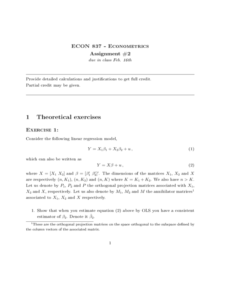
ECON 837 - Econometrics
Assignment #2
due in class Feb. 16th
Provide detailed calculations and justications to get full credit.
Partial credit may be given.
1 Theoretical exercises
Exercise 1:
Consider the following linear regression model,
Y = X1 β1 + X2 β2 + u ,
(1)
Y = Xβ + u ,
(2)
which can also be written as
where X = [X1 X2 ] and β = [β1′ β2′ ]′ . The dimensions of the matrices X1 , X2 and X
are respectively (n, K1 ), (n, K2 ) and (n, K) where K = K1 + K2 . We also have n > K .
Let us denote by P1 , P2 and P the orthogonal projection matrices associated with X1 ,
X2 and X , respectively. Let us also denote by M1 , M2 and M the annihilator matrices1
associated to X1 , X2 and X respectively.
1. Show that when you estimate equation (2) above by OLS you have a consistent
estimator of β2 . Denote it β̂2 .
1 These
are the orthogonal projection matrices on the space orthogonal to the subspace dened by
the column vectors of the associated matrix.
1
2. What is the asymptotic distribution of β̂2 ?
3. How does the asymptotic variance of β̂2 compare with the variance of β̂2 when
the sample size is xed?
Exercise 2:
Consider the following model:
yt = β1 × t + ut
where yt are time series observations, the error terms ut are i.i.d., and the observations
go from t = 1 to t = T . In other words, there is a single explanatory variable and it is
time itself.
1. Show that the OLS estimator of β1 is consistent. Denote it β̂1 .
2. Derive the asymptotic distribution of β̂1 including its rate of convergence, and its
asymptotic variance. Make sure you justify your steps by quoting the appropriate
statistical results and required assumptions.
3. Consider the residuals of the above OLS estimation to estimate the variance of
ut . Can we get a consistent estimator by using the usual formula for the sampling
variance? Justify your answer.
2 Computational exercise
Exercise 3:
In this exercise, we want to study and illustrate the rate of convergence of the estimator
considered in Exercise 2. The model is
yt = β1 xt + ut .
The error term ut is i.i.d. N (0; 1). The true value of β1 is 1.
2
1. Consider a rst experiment where the regressor xt consists in i.i.d. draws from a
uniform distribution on the [0; 10] interval.
(a) For a given sample size T , simulate observations for X , simulate the error
term U , then, with X , U , and using β1 = 1, compute Y . With the simulated
Y and X , estimate β1 by OLS and save this value. Now repeat this exercise
4999 more times (simulate X and U , compute Y , compute and save β̂1(1) ).
(b) Compute the sample mean and variance from the 5,000 estimated values for
β1 .
(c) Do all this for 13 dierent sample sizes2 ,
T = 50, 100, 200, 300, · · · , 800, 900, 1000, 2500, 5000.
2. Consider now a second experiment where everything is the same as in the rst
experiment, except that you take xt = t with t = 1, · · · , T (instead of drawing
numbers from a uniform distribution). The estimator is denoted β̂1(2) . Repeat all
the simulations and computations you did in experiment 1.
3. In a table, report the dierent sample sizes and corresponding sample means and
variances for each experiment. Discuss these results, and especially the convergence rates of the two estimators. Are they consistent with the results found in
Exercise 2? Explain.
4. To further investigate the discrepancy between the two convergence rates, perform
the following regression of the log of the square-root of the ratio of the MonteCarlo variances of β̂1(2) and β̂1(1) on the log-sample size, that is
(
ln
(2)
V ar(β̂1 )
)1/2
= α + γ ln(Ti ) + ϵi
(1)
V ar(β̂1 )
(a) What do you expect the slope parameter to be equal to? Explain.
(b) Estimate the slope parameter. Discuss your result.
2 Consider
running a double 'for' loop: the outside loop with index i from 1 to 13 selecting the appropriate sample size; the inside loop with index j from 1 to 5,000 to do the simulation and estimation.
This is an extension of the simulation exercise done in your rst assignment.
3