Exam #1 Answer Key
Economics 435
Spring 2004
1
Airplanes
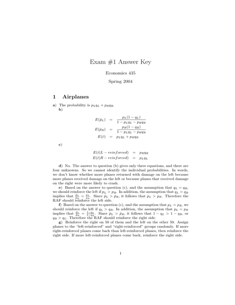
a) The probability is pL qL + pR qR .
b)
E(p̂L )
E(p̂R )
E(ĉ)
pL (1 − qL )
1 − pL q L − pR q R
pR (1 − qR )
=
1 − pL q L − pR q R
= pL q L + pR q R
=
c)
E(ĉ|L − reinf orced)
E(ĉ|R − reinf orced)
= pR q R
= pL q L
d) No. The answer to question (b) gives only three equations, and there are
four unknowns. So we cannot identify the individual probabilities. In words,
we don’t know whether more planes returned with damage on the left because
more planes received damage on the left or because planes that received damage
on the right were more likely to crash.
e) Based on the answer to question (c), and the assumption that qL = qR ,
we should reinforce the left if pL > pR . In addition, the assumption that qL = qR
implies that p̂p̂RL = ppRL . Since p̂L > p̂R , it follows that pL > pR . Therefore the
RAF should reinforce the left side.
f) Based on the answer to question (c), and the assumption that pL = pR , we
should reinforce the left if qL > qR . In addition, the assumption that pL = pR
1−qL
implies that p̂p̂RL = 1−q
. Since p̂L > p̂R , it follows that 1 − qL > 1 − qR , or
R
qR > qL . Therefore the RAF should reinforce the right side.
g) Reinforce the right on 50 of them and the left on the other 50. Assign
planes to the “left-reinforced” and “right-reinforced” groups randomly. If more
right-reinforced planes come back than left-reinforced planes, then reinforce the
right side. If more left-reinforced planes come back, reinforce the right side.
1
2
Income and life expectancy
a) The null hypothesis is
H0 : β2 = 0
The alternative is:
H1 : β2 6= 0
The test statistic is:
t=
β̂2
ˆ
sd(β̂2
Under the null, its asymptotic distribution is N (0, 1) implying we should reject
the null if |t| > 1.96. The actual value of the test statistic is:
−0.0353
= 6.08
0.0058
So we reject the null. The relationship is not linear.
b) The effect will be (1.9375 + 2 ∗ (−0.0353) ∗ GDP )∆GDP
c) The change will be 1.9375 ∗ (4.733 − 0.490) − 0.0353 ∗ (4.7332 − 0.4902 ) =
7.43 years. So moving up to the median income is predicted to increase life
expectancy to around 46.43 years.
3
The mode
a) Using the hint, we note that:
M = arg max E[I(x = z)]
z∈K
Applying the analog principle, we get
n
M̂ = arg max
z∈K
1X
I(xi = z)
n i=1
In other words, pick M̂ to be the value of x that appears most frequently in the
sample.
b) This estimator is biased. Suppose that n = 1, K = {0, 1}, and f (1) =
0.75, f (2) = 0.25. Note that the population mode is 1. Now we find the expected
value of M̂ . With probability 0.75, we will have x1 = 1 and thus M̂ = 1. With
probability 0.25, we will have x1 = 0 and thus M̂ = 0. Therefore, for a sample
of size 1, E(M̂ ) = 0.75 6= M .
c) This estimator is consistent. Let the parameter vector (θ1 , θ2 , . . . , θk ) =
Pn
(f (K1 ), f (K2 ), . . . , f (Kk )) and let θ̂i = i=1 I(xi = Ki ). First, note that as a
consequence of the law of large numbers,
plim θ̂i = θi
2
Applying the Slutsky theorem,
plim M̂
=
plim max(θ̂1 , θ̂2 , . . . , θ̂k )
= max(plim θ̂1 , plim θ̂2 , . . . , plim θ̂k )
= max(θ1 , θ2 , . . . , θk )
= M
d) No. Consider the example we used for part (b) of the question. No
matter what value for n, the distribution of M̂ will take on one of only two
points. This will still be true if we subtract E(M̂ ) and divide by SD(M̂ ). So
this distribution cannot converge to a continuous distribution like the N (0, 1).
3